Download
1 / 16
170 likes | 334 Vues
Cash Flow. +. R. P. F. time. -. Discounted Cash Flow Analysis (aka Engineering Economy). Objective: To provide economic comparison of benefits and costs that occur over time Assumptions: Future benefits and costs can be predicted All Benefits, Costs measured in money

E N D
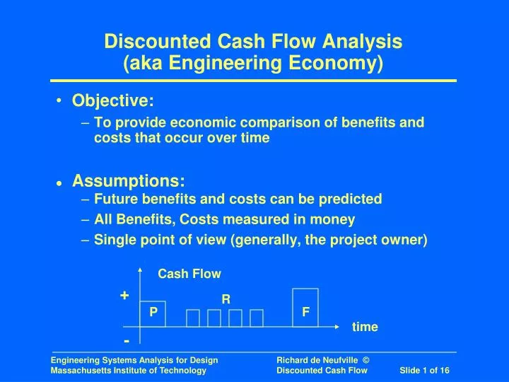
Cash Flow + R P F time - Discounted Cash Flow Analysis(aka Engineering Economy) • Objective: • To provide economic comparison of benefits and costs that occur over time • Assumptions: • Future benefits and costs can be predicted • All Benefits, Costs measured in money • Single point of view (generally, the project owner)
Issue - Value over time • Money now has a different value than the same amount at a different date • Comparable to – but not equal to – interest rate • Proper name: Discount Rate, r because future benefits/costs are reduced… (that is, “discounted”) to compare with present
Formulas for N Periods • Single amounts a) Future Amount = P (1 + r)N = P (caf) caf = Compound Amount Factor b) Present Amount = F/caf 1/caf = Present Worth Factor • Finite Series c) F = i R (1 + r)i = R [(1 + r)N - 1] / r d) R = P (crf) = [P*r (1+r) N ] / [(1 + r) N - 1] crf = Capital Recovery Factor
Formulas for N Periods (cont’) • Infinite Series 1 << (1 + r)N => (1+ r)N / [(1 + r)N - 1] => 1 => crf = r • Small Periods (1 + r)N ==> erN
Present Value Analysis • Present Value Analysis puts all future amounts on a common basis, typically “the present” • It may be some other reference year that is convenient, such as year of proposed investment • “Net” Present Value is the total of the present values of all future amounts, typically: Revenues – Costs = Net Amount • Referred to as “NPV”
Example Application of Present Value Analysis All by spreadsheets! Example:
Higher Discount rates => smaller value of future benefits discourages projects with long pay back periods project advocates try to minimize discount rate Examples: Massive Dams ; Airports; Aircraft projects Argument over Discount rates Often very difficult politically Not hard from technical perspective Generally higher than politicians want, for example, US Government base case before 2000 was 7%, but under current administration it is ~5% (see later slides) MORE DISCUSSION NEXT WEEK Effect of Different Discount Rates
US Govt base position on Discount rate (OMB Circular A-94,1992,revised yearly) 1. Base-Case Analysis. Constant-dollar benefit-cost analyses of proposed investments and regulations should report net present value and other outcomes determined using a real discount rate of 7 percent. This rate approximates the marginal pretax rate of return on an average investment in the private sector in recent years. Significant changes in this rate will be reflected in future updates of this Circular. 2. Other Discount Rates. Analyses should show the sensitivity of the discounted net present value and other outcomes to variations in the discount rate. The importance of these alternative calculations will depend on the specific economic characteristics of the program under analysis. For example, in analyzing a regulatory proposal whose main cost is to reduce business investment, net present value should also be calculated using a higher discount rate than 7 percent. http://www.whitehouse.gov/omb/circulars/a094/a094.html (accessed pre 2000)
Graphical view of Effect of Different Discount Rates and Lengths of Time
Discount Rate Approximation • To appreciate effect of discounting: “Rule of 72” or “Rule of 70” erN = 2.0 when rN = 0.72 (actually = 0.693) • Therefore, present amount doubles when future amount halves rN = 72 with r expressed in percent • Examples • When would $1000 invested at 10% double? • What is, at 9%, the value of $1000 in 8 years?
Longer Periods of Benefits Increase Present Values Increment depends on discount rate What length of time matters? For US Government Rate, not much over 30 years For Rates commonly used in business (15 to 20%), anything over 20 years has little value Exception: If future benefits grow exponentially, they may compensate for discounting of future revenues Effect of Different Time Horizons
Current US Government position on Discount rate (OMB Circular A-94) Provides 2 rates: Nominal represents future purchasing power; reflects inflation Real represents constant-dollar; assumes no inflation => Difference implies assumed rate of inflation These rates change yearly (as of last several years) These rates differ according to period – lower rates for shorter periods Note: assumed rate of inflation differs by period (See next slides)
Discount rates by OMB Circ. A-94, Appendix C[Ref: www.whitehouse.gov/omb/circulars/a094/a094_appx-c.html]
Guidelines appear precise (2 significant figures) But they are highly variable from year to year (see next slide), so analysis done in year N can be significantly off in year N+1 Would seem to be political, as evidenced by comparing rates from last 6 years with those given before 2000 (see slide 8) However…
Formulas Simple Especially by Spreadsheets Discount rate is key issue High rates recommended (but see later presentations) Longer term benefits not large Summary