Download
1 / 18
180 likes | 301 Vues
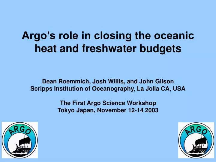
Argo’s role in closing the oceanic heat and freshwater budgets Dean Roemmich, Josh Willis, and John Gilson Scripps Institution of Oceanography, La Jolla CA, USA The First Argo Science Workshop Tokyo Japan, November 12-14 2003. Argo’s role in closing the oceanic heat and freshwater budgets.

E N D
Argo’s role in closing the oceanic heat and freshwater budgetsDean Roemmich, Josh Willis, and John GilsonScripps Institution of Oceanography, La Jolla CA, USAThe First Argo Science WorkshopTokyo Japan, November 12-14 2003
Argo’s role in closing the oceanic heat and freshwater budgets • A primary objective of global ocean observations is to close the mass, heat, and freshwater budgets of the oceans. • Argo implementation will enable improved estimates of ocean heat and freshwater storage and transport on seasonal, interannual and decadal timescales. • Examples are presented to illustrate the present global reach and enormous potential of Argo data: • Example 1: Global seasonal heat and freshwater storage from Argo. • Example 2: Global interannual ocean heat content from satellite and in situ datasets, including Argo. • Example 3: Closing interannual heat budgets.
Example 1: Global seasonal storage from Argo. Global estimates of seasonal heat and freshwater storage are made from the present Argo array - subtracting heat or salt content at 10-day intervals for each float, and averaging by latitude. Winter At right, plots of density, temperature, and salinity versus depth for a single float’s 2-year record are colored according to season. The fresher group of summer salinities occurred during the first year. The float’s trajectory is shown together with contours of mean 250-m T and S from WOA01. Note that, unlike temperature, the interannual variability in freshwater storage is as large as the seasonal cycle. Summer See poster by Gilson and Roemmich
Global seasonal heat storage, from 34,000 Argo profile-pairs. (Black) Argo heat storage, zonally averaged. (Red) NCEP air-sea exchange, 3-year average. (Lt Blue) NCEP subsampled at place and time of Argo profile. (Green) No. of profile pairs in average value. April - June Oct - Dec W/m2 See poster by Gilson and Roemmich
Global seasonal freshwater storage, from 29,000 Argo profile-pairs. The S/N ratio is much lower than for heat because seasonal variability in freshwater cycle does not dominate the frequency spectrum. (Black) Argo freshwater storage, zonally averaged. (Red) NCEP P-E, 3-year average. (Blue) NCEP P-E subsampled. (Green) No. of profile pairs in average value. Jan - Mar Jul - Sep See poster by Gilson and Roemmich mm/day
Regional heat storage – the Northeast Pacific. Plots at left show the heat balance for the Northeast Pacific, from 46.4 float years located north of 45oN and east of 150oW. In the upper panel, monthly values of spatially-averaged NCEP heat gain by the ocean (red) are compared to estimates from Argo (black). There is good correspondence not only in the seasonal cycle, but on a monthly basis, with somewhat greater amplitude of monthly variability in the Argo data. The heat flux values of the upper panel are integrated in time to produce heat content in the lower panel. The green line removes a mean value of 16 W/m2 from air-sea flux, presumed to be due to ocean heat flux divergence. See poster by Gilson and Roemmich, and presentation by Freeland and MacDonald
2000 Example 2: Global interannual ocean heat content. Willis, Roemmich, and Cornuelle (2003, In preparation) combined altimetric height and profile data (Argo + XBT + CTD) to estimate interannual variability in global ocean heat content and to judge the impact of Argo implementation. The technique makes a first guess using the AH/heat content correlation (synthetic method), then corrects it when and where data are available. No. of T-profiles
10-year trend in global ocean heat content, 0 – 750 m. The largest heat gain is about 40oS, where more profile data are needed. Profile data alone Zonal average 0 4 W/m2 Willis et al, 2003 AH plus profile data 0 4 W/m2
The zonally averaged temperature trend (oC/yr) is shown as a function of latitude and depth. The mid-latitude signals penetrate deeper than the tropical ones, and warming at 40oS is more widespread than at 40oN. Willis et al, 2003
At 40oS in the eastern Tasman Sea, a 12-year record from High Resolution XBT sections confirms the 0 – 800 m warming signal. Argo is needed for observation of such patterns on a global basis. Sutton and Bowen, 2003
Willis et al, 2003 • The Pacific ENSO signal spreads poleward from the equator. • The 40oS trend is strong in the Pacific and Indian.
2.3 mm/yr 1.8 mm/yr An important issue is the separation of sea level rise into steric expansion and (ground) ice melting components. Argo can detect steric expansion and eventually, salinity dilution due to ice melting. About 65% of the sea level rise estimated from AH and sea level gauges during the 10-year period is attributed to steric expansion. Willis et al, 2003
Example 3: Closing regional budgets. Heat content (J/m2) The interannual heat budget for the Tasman Box is estimated using a combination of datasets (Roemmich et al, 2003): - Storage from XBTs + CTDs + Argo, combined with AH - Transport from High Resolution XBT lines and AH - Air-sea flux from ECMWF surface analysis
Net northward transport Net eastward transport Net northward transport Variability in transport. Net transport (12-month running mean) across the faces of the Box, of water warmer than 12oC,results from the East Australian Current and recirculations. Variability in net transport is as large as the mean. The largest fluctuation was a period of low throughflow in late 1995, followed by high throughflow in 1997. Throughflow variability ~ 5 Sv Convergent variability ~ 1 Sv Roemmich et al, 2003
Closing the heat budget: Argo would reduce the error in heat transport by > 50% in this example – by providing 800 m reference velocity and 12oC isotherm depth. It would also enable the analogous E-P calculation. The objective is to reduce the errors to much smaller than the 30 W/m2 signal in this example. Ocean heat transport Storage ECMWF air-sea flux Residual calculation Roemmich et al, 2003
And diagnosing its variability: Roemmich et al, 2003 The throughflow transport is determined by wind-stress curl, which also affects SST via latent heat flux. The latter process dominates on interannual timescale, giving the unexpected result that SST minima correspond to throughflow maxima. The decadal balance may be different.
Conclusions (1): • The Argo array is already dense enough to resolve global seasonal variability in ocean heat content, and regional interannual variability in well-sampled locations. • Argo and altimetry are a powerful complementary combination for studies of global change; each one mitigates the limiting factors of the other. At the moment, southern hemisphere Argo is most in need of enhancement. • Argo will enable closure of regional heat and freshwater budgets with good signal-to-noise ratio. Systematic observations of the boundary currents is still needed.
Conclusions (2): Where are we headed? Many disparate datasets – altimetric height, scatterometer winds, Argo, etc., can be integrated using data assimilation models. At right is shown the Tasman regional heat budget from one such model (Stammer et al, 2003). It is necessary to proceed cautiously, measuring all components of the balance with high signal-to-noise ratio (on interannual time-scale and spatial scales of thousands of km) in order to test and improve the models. Right: Regional heat budgets from Stammer et al, 2003, ECCO assimilation