Download
1 / 19
190 likes | 309 Vues
Statistical Physics Approach to Understanding the Multiscale Dynamics of Earthquake Fault Systems. Theory. Systems composed of large number of simple, interacting elements. Statistical Physics Approach to Understanding the Multiscale Dynamics of Earthquake Fault Systems.

E N D
Statistical Physics Approach to Understanding the Multiscale Dynamics of Earthquake Fault Systems Theory
Systems composed of large number of simple, interacting elements Statistical Physics Approach to Understanding the Multiscale Dynamics of Earthquake Fault Systems Uninterested in small-scale (random) behaviour Use methods of statistics (averages!) Huge range of scale Phenomenology of dynamics
Overview • Motivation • Scaling laws • Fractals • Correlation length • Phase transitions • boiling & bubbles • fractures & microcracks • Metastability, spinodal line
Limitations to Observational Approach • Lack of data (shear stress, normal stress, fault geometry) • Range of scales: Fault length: ~300km Fault slip ~ m Fault width ~ cm
Scaling Laws log(y) = log(c) - b log(x) b>0 y = c x-b Why are scaling laws interesting? Consider interval (x0, x1) minimum of y is y1 = c (x1)-b maximum of y is y2 = c (x0)-b ratio y2/y1 = (x0/x1)-b now consider interval ( x0, x1) minimum of y is y1 = c (x1)-b maximum of y is y2 = c ( x0)-b ratio y2/y1 = (x0/x1)-b x0 x1 λx0 λ x1 compare with: y = ex/b, b>0 on (x0, x1), y1 = ex0/b, y2 = ex1/b y2/y1 = e(x1-x0)/b on ( x0, x1), y1 = e x0/b, y2 = e x1/b y2/y1 = e (x1-x0)/b → ratio independent of scale λ! → power-law relation ≈ scale-free process
Earthquake scaling laws Gutenberg-Richter Law • Log Ngr(>m) = -b m + a • m = magnitude, measured on logarithmic scale • Ngr(>m) = number of earthquakes of magnitude greater than m occurring in specified interval of time & area • Valid locally & globally, even over small time intervals (e.g. 1 year) Omori law: dNas/dt = 1/t0 (1+t/t1)-p Nas = number of aftershocks with m>specified value t = time after main shock Benioff strain: i.e. intermediate EQ activity increases before big EQ N = number of EQs up to time t ei = energy release of ith EQ
Fractals Fractal = self-similar = scale-free e.g. Mandelbrot set Fractals are ubiquitous in nature (topography, clouds, plants, …) Why? c.f. self-organized criticality, multifractals, etc.
Correlation Length Correlations measure structure On average, how different is f(x) for two points a distance L apart? L Let correlation length = scale where correlation is maximal L Lc L Correlation length ~ largest structure size Correlation length → ∞ ~ all scales present = scale-free
Phase transition model… Let’s look at earthquakes as phase transitions!
Phase diagram of a pure substance: coexistence of liquid and vapor phases! Isothermal decrease in pressure Liquid boils at constant P Vapor equilibrium curve Formation of metastable, superheated liquid Reduction in P, leads to isothermal expansion Spinodal curve: limit of stability. No superheating beyond!!! Explosive nucleation and boiling (instability) at constant P,T
isotherms pressure volume s’more about stability… why a spinodal line? Consequence of… Van der Waals equation (of state) (real gas) Ideal Gas Law correction for the real volume of the gas molecules, volume enclosed within a mole of particles correction term for intermolecular force, attraction between particles isotherms pressure volume Incompressible fluid (liquid): at small V and low P: isotherms show large increase in P for small decrease in V Metastable region: 2-phase coexistence at intermediate V and low P with horizontal isotherms compressible fluid (gas): at large V and low P: isotherms show small decrease in P for large decrease in V
Limit of stability! The spinodal line is interesting! It acts like a line of critical points for nucleating bubbles
Now let’s look at brittle fracture of a solid as a phase change… Damage occurs along constant strain path until stress is reduced to yield stress (IH)… similar to constant volume boiling (DH) Damage occurs at constant stress or pressure Undergoes phase change at B Let’s look at a plot of Stress vs. Strain… Elastic solid rapidly loaded with constant stress ( < yield stress) Elastic solid strained rapidly with a constant strain ( < yield strain) Deforms elastically until failure at B
When damage occurs along a constant strain path… We call it stress relaxation! Applicable to understanding the aftershock sequence that follows an earthquake Rapid stress! Rapid stress! earthquake Rapid stress! Rapid stress! If rapid stress is greater than yield stress: microcracks form, relaxing stress to yield stress
Time delay of aftershock relative to main shock = time delay of damage Why? Because it takes time to nucleate microcracks damage occurs in form of microcracks. when Damage is accelerated strain, leading to a deviation from linear elasticity.
How do we quantify derivation from linear elasticity? a damage variable!! as failure occurs as increases : brittle solid weakens due to nucleation and coalescence of Microcracks.
Spinodal Line nucleation Metastable region coalescence Increasing correlation length phase change
Metastability – an analogy Consider a ball rolling around a ‘potential well’ Gravity forces the ball to move downhill If there is friction, the ball will eventually stop in one of the depressions (A, B, C) What happens if we now perturb the balls? (~ thermal fluctuations) B is globally stable, but A & C are only metastable A C B If we now gradually make A & C shallower, the chance of a ball staying there becomes smaller Eventually, the stable points A & C disappear – this is the limit of stability, the spinodal Tomorrow, we will consider a potential that changes in time