Infinitely repeated games The concept of present value (see pp.14-18):

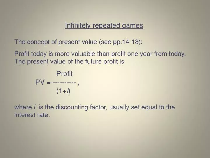
1. Infinitely repeated games The concept of present value (see pp.14-18): Profit today is more valuable than profit one year from today. The present value of the future profit is Profit PV = ---------- , (1+i) where i is the discounting factor, usually set equal to the interest rate.

2. A firm that is believed to exist and earn profits infinitely into the future has the present value of (Such an expression is called an infinite series.)

3. A couple of useful facts about infinite series: If the profits, π, are the same in each period and we start counting with the present period, then If the first period in the series is “a year from now”, then

4. Airline pricing game, revisited What if this game is played repeatedly?

5. Firms use “trigger strategies” – strategies contingent on the past play of a game (a certain action “triggers” a certain response). Suppose both firms are currently keeping their prices high. An example of a trigger strategy: “I will continue to play “HIGH” as long as you are playing “HIGH”. Once you cheat by playing “LOW”, I will play “LOW” in every period thereafter.” If firm 1 continues to cooperate, its present value is

6. Firms use “trigger strategies” – strategies contingent on the past play of a game (a certain action “triggers” a certain response). Suppose both firms are currently keeping their prices high. An example of a trigger strategy: “I will continue to play “HIGH” as long as you are playing “HIGH”. Once you cheat by playing “LOW”, I will play “LOW” in every period thereafter.” If firm 1 continues to cooperate, its present value is

7. If firm 1 cheats, its present value is Firm 1 will prefer to cooperate if or or 6 i+ 6 > 8 i + 3 If the rate of discounting is less than 66.7%, then both firms prefer to cooperate  3 > 2 i i < 66.7%  

8. Another example of a trigger strategy: Quality choice by a firm. The good can be purchased repeatedly.

9. A trigger strategy by consumers that can support the mutually beneficial outcome: “I will buy your product as long as you produce high quality. Once you produce low quality, I will never buy your product again”

11. Economics of incomplete information Traditional microeconomic analysis deals with economic agents making decisions under complete information. Examples of such assumptions: Consumers know the utility they get from a good; Firms know demand schedules; Firms know each others’ prices; and so on. Real life is more complicated and less certain.

12. Comparing projects with uncertain outcomes Every project has two characteristics, the expected value and the degree of risk. A certain outcome = no risk. The expected value, or the mean: Computed as the weighted sum of all possible payoffs (“weighted” = multiplied by the probabilities of each respective outcome): E[x] = q1x1 + q2x2 + … + qnxn, where xi is payoff i, qiis the probability that payoff i occurs, and q1 + q2 + … + qn= 1.

13. Variance (a measure of risk): • The sum of (the probabilities of each outcome multiplied by the squared differences between the value of the random variable and its mean: Var = q1(x1 – E[x])2 + q2(x2 – E[x])2 + … + qn(xn – E[x])2 The standard deviation, σ, is the square root of the variance. The larger the variance (or the standard deviation), the riskier the project. (For events occurring with certainty, Var = 0)

14. How much would you be willing to pay for a lottery ticket that pays $100 with a 50% probability and nothing with a 50% probability? I personally would pay… $30 What is the expected value of this lottery? • E[x] = q1x1 + q2x2 = 0.5 ∙ 100 + 0.5 ∙ 0 = $50 Why the difference?

15. The attitude to risk may vary. • Individuals who prefer less risk to more risk, all other things being equal, are called “risk averse”. It is believed that most people belong to this group. • Those who don’t care about the degree of risk and care only about the expected value are called “risk neutral”. • Individuals who prefer more risk to less risk, all other things being equal, are called “risk preferring”, or “risk loving”. • (Sort of an anomaly.) In the example above, the person in question is . . . risk averse.

16. “Risk premium” – the minimum reward that would induce a risk averse person to accept risk while preserving the same expected value. Alternatively, risk premium is the maximum amount of money an individual will be willing to pay to replace an uncertain situation with a certainty situation that has the same expected value. Risk premium depends on the characteristics of the lottery as well as on individual preferences. In the example above, my risk premium is $20. I will pay only $30 for a lottery; in other words, will trade certain $50 for this lottery only for a premium of 50 – 30 = $20

17. Project selection Suppose we have two projects: A: expected value = $1000, Var = 5000 B: expected value = $1000, Var = 1500 Which one will each type choose? Risk averse – Risk neutral – Risk loving – will choose B indifferent; either A or B will choose A

18. What if the expected values differ as well? A: expected value = $1200, Var = 5000 B: expected value = $1000, Var = 1500 Everyone prefers higher expected value to lower expected value, all other things being equal. Risk preferences of each type are the same as on the previous slide.

19. What can a risk averse individual do to reduce risk? • 1. Be informed. • Useful information has value!!! • 2. Diversify.

20. Diversification, or “spreading the risk”. You are considering investing $100 into one or two assets (stocks, for concreteness). Each stock is worth $50 now, and you believe that within the next three months its value can with equal probability either increase to $80 or drop to $40. For now, let us assume that what happens to one stock is not correlated to what happens to the other one.

21. Expected value of the investment: If you invest in the shares of only one of the companies: E[x] = 2 (0.5·80 + 0.5·40) = $120 If you buy one share of each of the two companies: E[x] = (0.5·80 + 0.5·40) + (0.5·80 + 0.5·40) = $120

22. The variance: If you invest in one company: Var = 0.5 (160 – 120)2 + 0.5 (80 – 120)2 = • = 0.5·1600 + 0.5·1600 = 1600 If you invest in both… Possible outcomes: W/prob ¼ both stocks go up, x = $160 W/prob ¼ stock A goes up, stock B falls, x = $120 W/prob ¼ stock B goes up, stock A falls, x = $120 W/prob ¼ both stocks fall, x = $80 • Var = 0.25 (160 – 120)2 + 0.5 (120 – 120)2+ 0.25 (80 – 120)2 = • = 0.25·1600 + 0.25·1600 = 800

23. If the payoffs from two assets are negatively correlated, then diversification becomes even more attractive. • Example: Two companies compete for a large government contract. After the winner is announced, the winner’s stock goes up and the loser’s stock falls. When firms undertake many projects at the same time, it is best for them to be risk neutral. Moreover, shareholders WANT managers to act in a risk-neutral manner (to care only about expected values).

24. Summary: • Everyone prefers a higher expected value to a lower expected value. • Most individuals are risk averse. This means they prefer less risk to more risk, provided the expected value stays the same. If one project offers a higher expected value and a higher risk at the same time, then we need more information to tell which of the two will a risk averse person choose. • Firms can be assumed to be risk neutral. They evaluate projects based solely on their expected values.

25. Pricing and output decisions under uncertainty Consider a modification of problem 4 on p.469. You are the manager of a firm that sells soybeans in a perfectly competitive market. Your cost function is C(Q) = 2Q +2Q2. Due to production lags, you must make your output decision prior to knowing what the market price is going to be. You believe that there is a 25% chance the market price will be $120 and a 75% chance it will be $160. What is the optimal quantity of output ? • The good news: • All the rules we have learned before (MR=MC, etc.) still apply but “expected” appear in them as needed. • Let’s do it step by step.

26. Normally, the rule we’d apply would be P=MC. Here, we replace P with its expected value, E(P). • Calculate the expected market price. • E(P) =0.25·120 + 0.75·160 = 30 + 120 = 150 b. What output should you produce to maximize expected profits? • E(P) = MC TC = 2Q +2Q2 therefore MC = 2 + 4Q • 150 = 2 + 4Q • 148 = 4Q • Q = 37

27. c. What are your profits under each outcome and the expected profits? You produce Q=37 which determines your cost, TC = 2·37 + 2·372 = 74 + 2738 = $ 2,812 If P = 120, your profit is = 120·37 – 2812 = $ 1,628 (happens w/prob ¼ ) If P = 160, your profit is = 160·37 – 2812 = $ 3,108 (happens w/prob ¾ ) Expected profit = ¼ · 1628 + ¾ · 3108 = $ 2,738

28. Looks like in one case we are underproducing and in the other case – overproducing. Wouldn’t it be better to bet on the most likely outcome? P = 160 MC = 2 + 4 Q 4 Q = 158 Q = 39.5 and TC = 2·39.5 + 2·39.52 = $ 3,199.50 If P = 160, our profit = 160·39.5 – 3199.50 = $ 3,120.50 If P = 120, our profit = 120·39.5 – 3199.50 = $ 1,540.50 Expected profit = ¼ · 1540.5 + ¾ · 3120.5 = $ 2,725.50

29. The same approach can be extended to the imperfectly competitive market case. • Consider the following problem: • A firm with market power produces at constant marginal (and average) cost of $1. There is a 50% chance of a recession and a 50% chance of an economic boom. • During a boom, the inverse demand for firm’s product will be • P = 10 – 0.5 Q • If there is a recession, the inverse demand will be P = 6 – 0.5 Q • The firm is risk neutral and must set output before demand is known. How much output should it produce to maximize expected profit?

30. Normally, we would look for the point where MR = MC. • This time, we will do E(MR) = MC. • There are two equally good ways to find expected marginal revenue: • Find expected demand, then expected marginal revenue: • Expected inverse demand: • E(P) = 0.5 (10 – 0.5 Q) + 0.5 (6 – 0.5 Q) = … = 8 – 0.5 Q • E(MR) = 8 – Q • 2. Find the marginal revenue under each scenario, then find the expected MR: • Boom: P = 10 – 0.5 Q MR = 10 – Q • Recession: P = 6 – 0.5 Q MR = 6 – Q • E(MR) = 0.5 (10 – Q) + 0.5 (6 – Q) = 8 – Q

31. The rest is trivial: • E(MR) = 8 – Q MC = 1 • E(MR) = MC • 8 – Q = 1 Q = 7 • If boom, then P = 10 – 0.5 Q = $6.50 • Profit = (P – AC) Q = (6.50 – 1) · 7 = $38.50 • If recession, then P = 6 – 0.5 Q = $2.50 • Profit = (P – AC) Q = (2.50 – 1) · 7 = $10.50 • Expected profit = 0.5 · 38.50 + 0.5 · 10.50 = $24.50 • Or directly: • “Expected price” given Q = 7 is E(P) = 8 – 0.5 Q = $4.50 • Exp.profit = (E(P) – AC) Q = (4.50 – 1) · 7 = $24.50

32. Consumer search for the best price and implications for the firm’s behavior General idea: A consumer samples several stores and obtains a price quote from each. The cost of obtaining each quote is the same. The total number of stores is large, so “drawing” one of them doesn’t affect the odds. After several quotes, you can always return to the store with the best price. It makes sense to continue searching as long as the (expected) benefit exceeds the cost of search.

33. Expected benefit: Joe wants to buy a DVD player. He thinks one-third of the stores charge $130 for a DVD player, one-third charge $100, and one-third charge $85. He sampled one store and the price was $100. What is the expected benefit from sampling another store? w/prob 1/3 next P = $85, a $15 benefit • w/prob 1/3 next P = $100, no benefit • w/prob 1/3 next P = $130, since he can return to the • first store, no benefit • Exp.benefit = (1/3)·15 = $5

34. How will the answer change if the best price found so far is $130? • w/prob 1/3 next P = $85, a $45 benefit • w/prob 1/3 next P = $100, a $30 benefit • w/prob 1/3 next P = $130, no benefit • Exp.benefit = (1/3)·45 + (1/3)·30 = $25

35. In general, if you sample a store and the price is high, the expected benefit from further search is greater (it makes more sense to keep searching). The lower the observed price, the more sense it makes to stop searching and buy. This principle holds even if the distribution of prices is not known.

36. Cost/benefit of continuing to search Exp.benefit of another search Cost of another search Price observed If observed P is at or below this level, we stop searching and buy

37. What happens if the cost of search increases? Cost/benefit of continuing to search Exp.benefit of another search Cost of another search Price observed Consumers are more likely to settle for higher prices.

38. What has happened with the advent of the Internet? • Search cost decreased; • As a result, consumers buy same goods at lower prices • Are all industries affected equally? • (Durable) consumer goods – very much so, • Groceries and expendable household items –

39. What has happened with the advent of the Internet? • Search cost decreased; • As a result, consumers buy same goods at lower prices • Are all industries affected equally? • (Durable) consumer goods – very much so, • Groceries and expendable household items – less; • Travel fares – affected a lot; • Industrial shipping rates – less. Why? • Insurance rates, phone rates – also affected a lot

40. Socially optimal risk sharing • If individuals are risk averse while firms are risk neutral, what is the optimal risk sharing between consumers and firms? • Getting out of risk has more value for consumers than for firms. • Therefore there is room for mutually beneficial exchange, where consumers reward the firm for accepting some of their risk for them. • Example: insurance industry.

41. Insurance companies are able to make money selling insurance because they may • - have better information about the odds than their clients; • - differ from clients in their attitude to risk; • - diversify. • The larger the group of the insured, the smaller the variance, hence the lower the risk.

42. Incomplete asymmetric information • “Asymmetric” in this case points at the fact that one party is less informed than the other. • The following analogy may be helpful: • A card game may be played under different rules: • All cards are dealt face up – complete information • Some (or all) cards are dealt face down – incomplete symmetric information. • Some (or all) cards are dealt face down but player can look at some of his own cards – incomplete asymmetric information.

43. An example of asymmetric information: Sellers know product quality, buyers do not. The only way for buyers to find out the true value is to try the product. (“Experience goods”) Under certainty, the rule for rational behavior is: Buy if Value > P, where “value” (a.k.a. “utility”) stands for the subjective value the buyer gets from the product. Under uncertainty, it becomes Buy if Exp. Value > P (for a risk neutral consumer) or Buy if Exp. Value – risk premium > P (for a risk averse consumer)

44. Say the product has a value of $100 for a consumer if it works as expected/promised. • The consumer believes that there is • a 90% chance the product will deliver services; • a 10% chance it will break down immediately (value = 0). • Up to what price will a risk neutral consumer pay for the product? • Max P = Exp Value = 0.9·100 + 0.1· 0 = $90 • What happens if the consumer is risk averse? • Max P = $90 – risk premium < $90 • If buyers’ subjective valuations of the good are below the producer’s cost of making it, the market breaks down – nothing will be sold.  • Both buyers and sellers are hurt by that.

45. Example: The market for “lemons” (Akerlof, 1973) analyzes the market for “lemons”, or cars with hidden defects. Asymmetric information is reflected in the fact that the quality of cars in the market is known to sellers but not to buyers. There are two types of used cars offered for sale in the market, 1,000good cars and 1,000 “lemons”.

46. The number of potential buyers exceeds the number of cars available (a case of “sellers’ market”). All buyers are identical – each of them will pay up to $1,000 for a lemon and $2,000 for a good car. (Those numbers are also called “reservation prices”.) The sellers’ “reservation price” (the lowest price they would agree to sell for) is $800 for a lemon and $1600 for a good car.

47. Case 1. Symmetric complete information – the true quality of each car is known to both parties. We have two separate markets: P P 2000 2000 P=$2000 1600 1600 P=$1000 1000 1000 800 800 Q Q 1000 1000 Good cars Lemons All cars are sold.

48. Case 2. Symmetric incomplete information – the true quality of a particular car is not known to anybody. Each car is either a good one (with a 50% probability) or a lemon (with a 50% probability). Neither buyers nor sellers can tell one from another. For simplicity, we are going to assume both sides are risk neutral. Therefore they base their reservation prices on expected values. • For sellers, EV = 0.5 ∙ 1600 + 0.5 ∙ 800 = $1,200 • For buyers, EV =0.5 ∙ 2000 + 0.5 ∙ 1000 = $1,500

49. P 2000 1500 1200 1000 800 Q 1000 2000 Equilibrium price = $1500 Equilibrium quantity = 2000

50. Case 3. Asymmetric incomplete information – sellers know the quality, buyers don’t. For buyers, the situation is the same as in the previous case – they will pay $1500 for any car. Sellers, however, can tell good cars from lemons, and their reservation price is different for each category. P 2000 1500 1200 1000 800 Q 1000 2000