Download
1 / 54
540 likes | 584 Vues
Learn how to interpret image histograms and use them for improving color contrast and brightness in digital images. Understand the calculation process and practical applications for enhancing image quality.

E N D
Lecture 10Grey Level & Colour Enhancement (2) TK3813 Dr. Masri Ayob
Image Histogram • The histogram of an image is a table containing (for every gray level K) the probability of level K actuallyoccurring in the image • The histogram could also be viewed as a frequency distribution of gray level within the image. Calculation of an image histogram: Create an array histogram with 2b elements For all grey levels, I, do histogram[i]=0 End for For all pixel coordinates, x and y, do increment histogram[f(x,y)] by 1 End for
Image Histograms The histogram on the left is representative of an “under-exposed” image. It has very few “bright” pixels and doesn’t make good use of the full dynamic range available. The histogram on the left is representative of an “over-exposed” image. It has very few “dark” pixels and doesn’t make good use of the full dynamic range available. Contrast : Amount of difference between average gray level of an object and that of surroundings The histogram on the left is representative of an “poor contrast” image. It has very few “dark” and very few “light” pixels. It doesn’t make good use of the full dynamic range available.
Image Histogram Added 150 to all pixels. If sum >255 at a pixel, gray level for that pixel is clipped to 255.
Image Histograms The histogram on the left is representative of an image with good contrast. It makes good use of the full dynamic range available. Brightness span of an image’s gray scale You can’t tell if an image is “good” just by looking at the histogram…but the histogram may give you a “tingly feeling” that something isn’t quite right.
Image Histogram The histogram seems “uneven” but the image has good contrast. It just happens to be a naturally “bright” image.
Image Histogram The histogram seems “squeezed” and it does indicate (in this case) that the image has poor contrast.
Test Your Knowladge Q: The image on the right was obtained by swapping the top and bottom halves of the image on the left. What is the relationship of the histograms of the two images? A: Both have the same histogram.
Cumulative Distribution Function • The CDF of an image is a table containing (for every gray level K) the probability of a pixel of level K OR LESS actually occurring in the image • The CDFcan be computed from the histogram as:
Image histogram Image CDF Cumulative Distribution Function • The CDF of represents a monotonically increasing function. • The derivative (slope) of the CDF is steep where there are lots of pixels and low where there are few pixels A function which is either entirely nonincreasing or nondecreasing. A function is monotonic if its first derivative (which need not be continuous) does not change sign.
Image histogram Image CDF Image histogram Image CDF Cumulative Distribution Function • The CDF of an image having uniformly distributed pixel levels is a straight-line with slope 1 (using normalized gray levels). The derivative of the CDF is constant.
Histogram Processing • Histogram of a digital image with gray levels in the range [0,L-1] is a discrete function h(rk) = nk • Where • rk : the kth gray level • nk : the number of pixels in the image having gray level rk • h(rk) : histogram of a digital image with gray levels rk
Histogram Processing • Basic for numerous spatial domain processing techniques • Used effectively for image enhancement • Information inherent in histograms also is useful in image compression and segmentation
Normalized Histogram • The probability of occurrence of gray level in an image is approximated by • The discrete version of transformation
Histogram Equalization • Thus, an output image is obtained by mapping each pixel with level rk in the input image into a corresponding pixel with level sk in the output image • In discrete space, it cannot be proved in general that this discrete transformation will produce the discrete equivalent of a uniform probability density function, which would be a uniform histogram
Histogram Equalization • As the low-contrast image’s histogram is narrow and centered toward the middle of the gray scale, if we distribute the histogram to a wider range the quality of the image will be improved. • We can do it by adjusting the probability density function of the original histogram of the image so that the probability spread equally
Histogram Equalization • Used to automatically distribute pixel valuesevenlythroughout the image • each gray level should appear with identical probability in the image • Often enhances an image, but not always
Histogram Equalization E.g., consider equalizing the following 4-bit image using the above formula:
Histogram Equalization Before After
Resulting image has increased dynamic range. Resulting histogram almost, but not completely, flat. Appears jagged and some gray levels unoccupied since finite number of gray levels are available. After Before
Histogram Equalization Example Source: Institue of Biotechnology, University of Helsinki, Mouse embryo 13 d pc, tissue section from molar tooth
before after Histogram equalization Example
No. of pixels 6 5 4 3 2 1 Gray level 4x4 image 0 1 2 3 4 5 6 7 8 9 Gray scale = [0,9] histogram Example
No. of pixels 6 5 4 3 2 1 Output image 0 1 2 3 4 5 6 7 8 9 Gray level Gray scale = [0,9] Histogram equalization Example Input image
Note • It is clearly seen that • Histogram equalization distributes the gray level to reach the maximum gray level (white) because the cumulative distribution function equals 1 when 0 r L-1 • If the cumulative numbers of gray levels are slightly different, they will be mapped to little different or same gray levels as we may have to approximate the processed gray level of the output image to integer number • Thus the discrete transformation function can’t guarantee the one to one mapping relationship
Note • Histogram processing methods are global processing, in the sense that pixels are modified by a transformation function based on the gray-level content of an entire image. • Sometimes, we may need to enhance details over small areas in an image, which is called a local enhancement.
Local Enhancement • Original image (slightly blurred to reduce noise) • global histogram equalization (enhance noise & slightly increase contrast but the construction is not changed) • local histogram equalization using 7x7 neighborhood (reveals the small squares inside larger ones of the original image. (a) (b) (c) • define a square or rectangular neighbourhood and move the center of this area from pixel to pixel. • at each location, the histogram of the points in the neighborhood is computed and histogram equalization transformation function is obtained. • another approach used to reduce computation is to utilize nonoverlapping regions, but it usually produces an undesirable checkerboard effect.
Explain the result in c) • Basically, the original image consists of many small squares inside the larger dark ones. • However, the small squares were too close in gray level to the larger ones, and their sizes were too small to influence global histogram equalization significantly. • So, when we use the local enhancement technique, it reveals the small areas. • Note also the finer noise texture is resulted by the local processing using relatively small neighborhoods.
Method Summary BufferedImage createCompatibleDestImage(BufferedImage src, ColorModel destCM) Creates a zeroed destination image with the correct size and number of bands. BufferedImage filter(BufferedImage src, BufferedImage dest) Performs a single-input/single-output operation on a BufferedImage. Rectangle2D getBounds2D(BufferedImage src) Returns the bounding box of the filtered destination image. Point2D getPoint2D(Point2D srcPt, Point2D dstPt) Returns the location of the corresponding destination point given a point in the source image. RenderingHints getRenderingHints() Returns the rendering hints for this operation. Implementation • Take a look at the built-in BuffereImageOp interface
Implementation public class StandardGreyOp implements BufferedImageOp { public BufferedImage filter(BufferedImage src, BufferedImage dest) { checkImage(src); if (dest == null) dest = createCompatibleDestImage(src, null); WritableRaster raster = dest.getRaster(); src.copyData(raster); return dest; } public BufferedImage createCompatibleDestImage(BufferedImage src, ColorModel destModel) { if (destModel == null) destModel = src.getColorModel(); int width = src.getWidth(); int height = src.getHeight(); BufferedImage image = new BufferedImage(destModel, destModel.createCompatibleWritableRaster(width, height), destModel.isAlphaPremultiplied(), null); return image; } // other methods here /// }
Implementation public class StandardGreyOp implements BufferedImageOp { // other methods here public Rectangle2D getBounds2D(BufferedImage src) { return src.getRaster().getBounds(); } public Point2D getPoint2D(Point2D srcPoint, Point2D destPoint) { if (destPoint == null) destPoint = new Point2D.Float(); destPoint.setLocation(srcPoint.getX(), srcPoint.getY()); return destPoint; } public RenderingHints getRenderingHints() { return null; } public void checkImage(BufferedImage src) { if (src.getType() != BufferedImage.TYPE_BYTE_GRAY) throw new ImagingOpException("operation requires an 8-bit grey image"); } }
Implementation public abstract class GreyMapOp extends StandardGrayOp { protected byte[] table = new byte[256]; // lookup table public abstract void computeMapping(int low, int high); public int getTableEntry(int i) { if (table[i] < 0) return 256 + (int) table[i]; else return (int) table[i]; } protected void setTableEntry(int i, int value) { if (value < 0) table[i] = (byte) 0; else if (value > 255) table[i] = (byte) 255; else table[i] = (byte) value; } public void computeMapping() { computeMapping(0, 255); } public BufferedImage filter(BufferedImage src, BufferedImage dest) { checkImage(src); if (dest == null) dest = createCompatibleDestImage(src, null); LookupOp operation = new LookupOp(new ByteLookupTable(0, table), null); operation.filter(src, dest); return dest; } }
Implementation public class SquareRootOp extends GreyMapOp { public SquareRootOp() { computeMapping(); } public SquareRootOp(int low, int high) { computeMapping(low, high); } public void computeMapping(int low, int high) { if (low < 0 || high > 255 || low >= high) throw new java.awt.image.ImagingOpException("invalid mapping limits"); double a = Math.sqrt(low); double b = Math.sqrt(high); double scaling = 255.0 / (b - a); for (int i = 0; i < 256; ++i) { int value = (int) Math.round(scaling*(Math.sqrt(i) - a)); setTableEntry(i, value); } } }
Implementation public class EqualiseOp extends GreyMapOp { public EqualiseOp(Histogram hist) throws HistogramException { float scale = 255.0f / hist.getNumSamples(); for (int i = 0; i < 256; ++i) table[i] = (byte) Math.round(scale*hist.getCumulativeFrequency(i)); } public void computeMapping(int low, int high) { // Does nothing - limits are meaningless in histogram equalisation } }
Implementation public final class Histogram implements Cloneable { public Histogram(); public Histogram(Reader reader); public Histogram(BufferedImage image) throws HistogramException; public void computeHistogram(BufferedImage image) throws HistogramException; private void accumulateFrequencies(BufferedImage image) throws HistogramException { if (image.getType() == BufferedImage.TYPE_BYTE_BINARY || image.getType() == BufferedImage.TYPE_USHORT_GRAY) throw new HistogramException("invalid image type"); Raster raster = image.getRaster(); if (image.getType() == BufferedImage.TYPE_BYTE_GRAY) { for (int y = 0; y < image.getHeight(); ++y) for (int x = 0; x < image.getWidth(); ++x) ++freq[0][raster.getSample(x, y, 0)]; } else { int[] value = new int[3]; for (int y = 0; y < image.getHeight(); ++y) for (int x = 0; x < image.getWidth(); ++x) { raster.getPixel(x, y, value); ++freq[0][value[0]]; ++freq[1][value[1]]; ++freq[2][value[2]]; } } }
PsuedoColoring • Artifical coloring (PsuedoColoring) can often enhance the presentation of image information • Replaces the gray-scale levels by an arbitrarilyselected palette or color bar
PsuedoColoring Color Tables are arbitrarily selected Palettes of colors. There are ways to automatically compute interesting palettes. Tables below were generated using offset sinusoidal waves in each of the RGB bands
PsuedoColoring The color tables below were generated by using offset sinusoids into each of the RGB bands.
Psuedo Coloring Example Weather satellite image. Note the way the colorized image brings out certain details that are difficult to distinguish in the original.
Psuedo Coloring Example Source: Institue of Biotechnology, University of Helsinki, Mouse embryo 13 d pc, tissue section from molar tooth The above tissue sample is colorized using two different color tables. Take your pick!
Image Averaging • consider a noisy image g(x,y) formed by the addition of noise (x,y) to an original image f(x,y) g(x,y) = f(x,y) + (x,y)
= image formed by averaging K different noisy images Image Averaging • if noise has zero mean and be uncorrelated then it can be shown that if
Image Averaging • Note: the images gi(x,y) (noisy images) must be registered (aligned) in order to avoid the introduction of blurring and other artifacts in the output image.
Example • a) original image • b) image corrupted by additive Gaussian noise with zero mean and a standard deviation of 64 gray levels. • c). -f). results of averaging K = 8, 16, 64 and 128 noisy images