Download
1 / 55
570 likes | 818 Vues
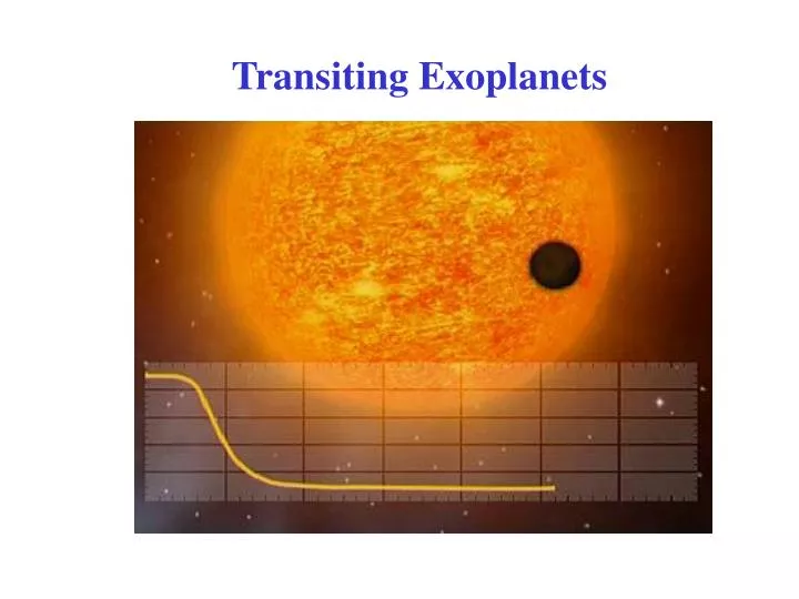
Transiting Exoplanets. Artie Hatzes Tel:036427-863-51 Email: artie@tls-tautenburg.de www.tls-tautenburg.de → Lehre → Vorlesungen → Jena. Tentative Schedule. 19. Oct: Introduction, Background, and Course overview 26. Oct: The Solar System, Basic Tools, Photometric technique

E N D
Artie Hatzes Tel:036427-863-51 Email: artie@tls-tautenburg.de www.tls-tautenburg.de→Lehre→Vorlesungen→Jena
Tentative Schedule 19. Oct: Introduction, Background, and Course overview 26. Oct: The Solar System, Basic Tools, Photometric technique 02. Nov: Sources of Noise and their Removal 09. Nov: Searching for transit signals in your data (Philipp Eigmüller) 16. Nov: Confirming the Nature of Transiting Planets 23. Nov: Modeling the Transit Curve (Szilard Czismadia) 30. Nov: Ground-based Surveys (Philipp Eigmüller) 07. Dec Results from the CoRoT Mission (Eike Guenther) 14. Dec: Results from the Kepler Mission 21. Dec: Spectroscopic Transits: Rossiter-McClaughlin Effect 04. Jan: Atmospheres of Transiting Planets 11. Jan Determination of Stellar Parameters (Matthias Ammler-von-Eiff) 18. Jan: Transit Timing Variations (Szilard Czismadia) 25. Jan: Space Missions: PLATO and TESS 01. Feb: Tidal Evolution of Close-in Planets (Martin Pätzold)
Literature • Contents: • Radial Velocities • Astrometry • Microlensing • Transits • Imaging • Host Stars • Brown Dwarfs and Free floating Planets • Formation and Evolution • Interiors and Atmospheres • The Solar System
Literature • Contents: • Our Solar System from Afar (overview of detection methods) • Exoplanet discoveries by the transit method • What the transit light curve tells us • The Exoplanet population • Transmission spectroscopy and the Rossiter-McLaughlin effect • Host Stars • Secondary Eclipses and phase variations • Transit timing variations and orbital dynamics • Brave new worlds By Carole Haswell
Contributions: • Radial Velocities • Exoplanet Transits and Occultations • Microlensing • Direct Imaging • Astrometric Detections • Planets Around Pulsars • Statistical Distribution of Exoplanets • Non-Keplerian Dynamics of Exoplanets • Tidal Evolution of Exoplanets • Protoplanetary and Debris Disks • Terrestrial Planet Formation • Planet Migration • Terrestrial Planet Interiors • Giant Planet Interior Structure and Thermal Evolution • Giant Planet Atmospheres • Terrestrial Planet Atmospheres and Biosignatures • Atmospheric Circulation of Exoplanets
Resources • The Extrasolar Planet Encyclopaedia (Jean Schneider): www.exoplanet.eu (note www.exoplanets.eu sends you to the Geneva Planet Search Program) • In 7 languages • Tutorials • Interactive catalog (radial velocity, transits, etc) • On line histrograms and correlation plots • Download data
Resources The Nebraska Astronomy Applet: An Online Laboratory for Astronomy http://astro.unl.edu/naap/ http://astro.unl.edu/animationsLinks.html http://astro.unl.edu/classaction/animations/extrasolarplanets/transitsimulator.html • Pertinent to Exoplanets: • Influence of Planets on the Sun • Radial Velocity Graph • Transit Simulator • Extrasolar Planet Radial Velocity Simulator • Doppler Shift Simulator • Pulsar Period simulator • Hammer thrower comparison
Exoplanets is a fast moving field, the best literature is the journals NASA Astronomical Data Systems Abstract Service: http://adswww.harvard.edu/ads_abstracts.html „Astronomy and Astrophysics Search“ Astro-ph preprint service: http://arxiv.org/
Rate of Transiting Exoplanet Discoveries Kepler-4b HD 209458b CoRoT-1b First OGLE Planet WASP-1b HAT-1b
Methods of Detecting Exoplanets • Doppler wobble - Velocity reflex motion of the star due to the planet: 459 planets • Transit Method - photometric eclipse due to planet: 184 planets • Astrometry - spatial reflex motion of star due to planet: 0 discoveries, 6 detections of known planets • Direct Imaging: 25 planets • Microlensing – gravitational perturbation by light: 13 planets • Timing variations – changes in the arrival of pulses (pulsars), oscillation frequencies, or time of eclipses (no transit timing variations): 12 planets
Historical Context of Transiting Planets (Venus) Transits (in this case Venus) have played an important role in the history of research of our solar system. Kepler‘s law could give us the relative distance of the planets from the sun in astronomical units, but one had to determine the AU in order to get absolute distances. This could be done by observing Venus transits from two different places on the Earth and using triangulation. This would fix the distance between the Earth and Venus.
Historical Context of Transiting Planets (Venus) From wikipedia Jeremiah Horrocks was the first to attempt to observe a transit of Venus. Kepler predicted a transit in 1631, but Horrocks re-calculated the date as 1639. Made a good guess as to the size of Venus and estimated the Astronomical Unit to be 0.64 AU, smaller than the current value but better than the value at the time.
Transits of Venus occur in pairs separated by 8 years and these were the first international efforts to measure these events. Le Gentil‘s observatory One of these expeditions was by Guilaume Le Gentil who set out to the French colony of Pondicherry in India to observe the 1761 transit. He set out in March and reached Mauritius (Ile de France) in July 1760. But war broke out between France and England so he decided to take a ship to the Coromandel Coast. Before arriving the ship learned that the English had taken Pondicherry and the ship had to return to Ile de France. The sky was clear but he could not make measurements due to the motion of the ship. Coming this far he decided to just wait for the next transit in 8 years. He then mapped the eastern coast of Madagascar and decided to observe the second transit from Manilla in the Philippines. The Spanish authorities there were hostile so he decided to return to Pondicherry where he built and observatory and patiently waited. The month before was entirely clear, but the day of the transit was cloudy – Le Gentil saw nothing. This misfortune almost drove him crazy, but he recovered enough to return to France. The return trip was delayed by dysentry, the ship was caught in a storm and he was dropped off on the Ile de Bourbon where he waited for another ship. He returned to Paris in 1771 eleven years after he started only to find that he had been declared dead, been replaced in the Royal Academy of Sciences, his wife had remarried, and his relatives plundered his estate. The king finally intervened and he regained his academy seat, remarried, and lived happily for another 21 years.
Historical Context of Transiting Planets (Venus) From wikipedia Mikhail Lomonosov predicted the existence of an atmosphere on Venus from his observations of the transit. Lomonosov detected the refraction of solar rays while observing the transit and inferred that only refraction through an atmosphere could explain the appearance of a light ring around the part of Venus that had not yet come into contact with the Sun's disk during the initial phase of transit.
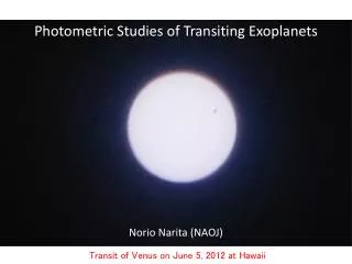
Venus limb solar
What can we learn about Planetary Transits? The radius of the planet The orbital inclination and the mass when combined with radial velocity measurements The Albedo from reflected light The temperature from radiated light Atmospheric spectral features In other words, we can begin to characterize exoplanets
R* DI The Planet Radius The drop in intensity is give by the ratio of the cross-section areas: DI = (Rp /R*)2 = (0.1Rsun/1 Rsun)2 = 0.01 for Jupiter Ground-based measurements can usually get a precision of about 0.01 mag
⅓ 1 ( 2pG Mp sin i ( P Ms⅔ (1 – e2)½ The Planet Mass The radial velocity amplitude is often called the K-amplitude In general from Kepler‘s law: Mp = mass of planet Ms = mass of star P = orbital period K= For circular orbits (often the case for transiting Planets): Where Mp is in Jupiter masses, P is in years, and Ms is in solar masses Mp sin i 28.4 K= m/s P1/3Ms2/3
Two important comments: 1) In the previous expressions I have made the approximation that Ms» Mp, otherwise replace Ms with (Mp + Ms) 2) For radial velocities we only measure the component of the orbital motion along the line-of-sight. Therefore we only can derive Mp x sin i, where i is the orbital inclination. But for transiting planets we know i. Thus transiting planets allow us to derive the true mass of the planet
Because you measure the radial component of the velocity you cannot be sure you are detecting a low mass object viewed almost in the orbital plane, or a high mass object viewed perpendicular to the orbital plane We only measure MPlanet xsin i i Observer
The Planet Atmosphere Two ways to characterize an exoplanet‘s atmosphere: • Spectra during primary eclipse: Chemical composition, scattering properties • Spectra during secondary eclipse: Chemical composition, temperature structure
90+q Porb = 2p sin i di / 4p = 90-q Useful Numbers: Transit Probability i = 90o+q q Rs = stellar radius a = semi-major-axis sin q = Rs/a = |cos i| –0.5 cos (90+q) + 0.5 cos(90–q) = sin q = Rs/a for small angles Note that for large planets you must replace Rs + Rp. If a =10 Rs for a Jupiter radius planet this changes the probability from 0.1 to 0.11. These would of course be a grazing transits.
2R* P (4p2)1/3 4p2 (as + ap)3 t P2 = 2p P2/3 M*1/3G1/3 G(ms + mp) Useful Numbers: The Transit Duration t = 2(R* +Rp)/v where v is the orbital velocity and i = 90 (transit across disk center) For circular orbits v = 2pa/P From Keplers Law’s: a = (P2 M*G/4p2)1/3 t1.82 P1/3 R* /M*1/3 (hours) In solar units, P in days
For more accurate times need to take into account the orbital inclination and the fact that you have a finite radius planet for i 90o need to replace R* with R: R2 + d2cos2i = R*2 R = (R*2– d2 cos2i)1/2 d cos i R* R
Transit Numbers from our Solar System N is the number of stars you would have to observe to see a transit, if all stars had such a planet
Useful Numbers: The Stellar Radius One can solve transit duration for the stellar radius: 0.55 t M1/3 R in solar radii M in solar masses P in days t in hours R = P1/3 Clearly the best estimate of the stellar radius comes from spectroscopy. However, the transit duration can be used 1) as a first estimate that you are dealing with a dwarf star and 2) a check on the spectroscopically derived stellar radius
2R* P (4p2)1/3 t 2p P2/3 M*1/3G1/3 Useful Numbers: The Stellar Density t1.09 G–⅓ P⅓ R* /M*⅓ t31.3 G P R*3 /M* t3 CP (rmean)–1 Where rmeanis the mean stellar density and is called the „transit stellar density“. This can be used as a „sanity check“ to compare with values determined from a formal spectral analysis. It also gives you the first hint on the evolutionary status of the star.
The Stellar Radius Radius as a function of Spectral Type for Main Sequence Stars A planet has a maximum radius ~ 0.15 Rsun. This means that a star can have a maximum radius of 1.5 Rsun to produce a transit depth consistent with a planet.
Along the Main Sequence Spectral Type Spectral Type DI/I Stellar Mass (Msun) Stellar Mass (Msun) The photometric transit depth for a 1 RJup planet
Along the Main Sequence Planet Radius (RJup) 1 REarth Stellar Mass (Msun) Assuming a 1% photometric precision this is the minimum planet radius as a function of stellar radius (spectral type) that can be detected
Probability of detecting a transit Ptran: Ptran= Porbx fplanetsx fstars x DT/P Porb = probability that orbit has correct orientation fplanets = fraction of stars with planets fstars = fraction of suitable stars (Spectral Type later than F5) DT/P = fraction of orbital period spent in transit
Estimating the Parameters for 51 Peg systems: P ~ 4 d fstars This depends on where you look (galactic plane, clusters, etc.) but typically about 30-40% of the stars in the field will have radii (spectral type) suitable for transit searches.
You also have to worry about late-type giant stars Example: A KIII Star can have R ~ 10 RSun DI = 0.01 = (Rp/10)2 → Rp = 1 RSun! Unfortunately, background giant stars are everywhere. In the CoRoT fields, 25% of the stars are giant stars Giant stars are relatively few, but they are bright and can be seen to large distances. In a brightness limited sample you will see many distant giant stars.
Estimating the Parameters for 51 Peg systems Fraction of the time in transit Porbit≈ 4 days Transit duration ≈ 3 hours DT/P 0.08
For each test orbital period you have to observe enough to get the probability that you would have observed the transit (Pvis) close to unity. For each field you have to observe enough to ensure that the probability is close to 1 that you would observe
Estimating the Parameters for 51 Peg systems Porb Period ≈ 4 days → a = 0.05 AU =10 Rסּ Porb 0.1 fplanets Although the fraction of giant planet hosting stars is 5-10%, the fraction of short period planets is smaller, or about 0.5–1%
E.g. a field of 10.000 Stars the number of expected transits is: Ntransits = (10.000)(0.1)(0.01)(0.3) = 3 Probability of a right orbital orientation Frequency of Hot Jupiters Fraction of stars with suitable radii So roughly 1 out of 3000 stars will show a transit event due to a planet. And that is if you have full phase coverage! CoRoT: looks at 10,000-12,000 stars per field and is finding on average 3 Hot Jupiters per field. Similar results for Kepler Note: Ground-based transit searches are finding hot Jupiters 1 out of 30,000 – 50,000 stars.
Catching a transiting planet is thus like playing Lotto. To win in LOTTO you have to • Buy lots of tickets → Look at lots of stars • Play often → observe as often as you can The obvious method is to use CCD photometry (two dimensional detectors) that cover a large field.
Large-field Searches from the Ground • OGLE (Optical Gravitational Lensing Experiment) • Started in 2001 with one a 1.3m telescope at Las Campanas • Originally a microlensing experiment • 35 x 35 arcmin2 field of view → look at galactic bulge • 5 million stars monitored → 52 000 with photometry better than 1.5% → 46 transits detected in first field • Typical magnitude V = 15-17 • 9 planets discovered including first transiting planet discovered with photometry
The first planet found with the transit method Until OGLE-TR-56 the shortest period planet that was found by the radial velocity method was 3 days.
Large-field Searches from the Ground • HAT/HATNet (Hungarian Automated Telescope) • Started in 2003 with one telescope • Currently 6 automated telescopes 4 at Whipple Observatory in Arizona and two in Mauno Kea • 2000 x 2000 pixels CCD with an 8 degree field of view • Precision 3-10 millimags at I = 8 – 11 • 32 planets discovered (2 shared with WASP)
Large-field Searches from the Ground • TRES (Trans-Atlantic Exoplanet Survey) • Started in 2000 with STARE (found first transiting exoplanet) • Three 0.1m telescopes (Arizona, California, Canary Islands) • CCD : 6 degree field of view • < 2 millimags for bright stars, 10 mmag for R ~ 12.5 • 5 planets discovered
HD 209458b • Mass = 0.63 MJupiter • Radius = 1.35 RJupiter • Density = 0.38 g cm–3
Large-field Searches from the Ground • WASP/SuperWASP (Wide Angle Search for Planets) • Started in 2004 as WASP, 2006 as SuperWASP • Each telescope uses eight 2k x 2k CCDs with a mosaic of 15 deg x 30 deg • First run observed 6.7 million objects • 4 mmag @V=9.5, 10mmag@V=12 • 65 planets discovered (2 shared with HAT) Rate: 50 million stars observed and 65 planets → 1 planet for every 1 000 000 stars
Large-field Searches from the Ground • XO • Started in 2003 • Aims at bright stars • Two 0.11m telescopes • 1k x 1k CCDs with a mosaic of 7 deg x 7 deg • First year of operation observed 7% of the sky and 100 000 stars • 10 mmag @V < 12 • 5 planets discovered Rate: 5 planets for every 100 000 stars 1 planet for every 20 000 stars