Download
1 / 21
300 likes | 680 Vues
State Space Analysis. Hany Ferdinando Dept. of Electrical Engineering Petra Christian University. Overview. State Transition Matrix Time Response Discrete-time evaluation. State Transition Matrix. The solution of . is.

E N D
State Space Analysis Hany Ferdinando Dept. of Electrical Engineering Petra Christian University
Overview • State Transition Matrix • Time Response • Discrete-time evaluation State Space 2 - Hany Ferdinando
State Transition Matrix The solution of is If the initial condition x(0), input u(t) and the state transition matrix F(t) are known the time response of x(t) can be evaluated State Space 2 - Hany Ferdinando
State Transition Matrix The F(t) is inverse Laplace Transform of F(s) and When the input u(t) is zero, then State Space 2 - Hany Ferdinando
State Transition Matrix From the equation above we can expand the matrix into (for example, two elements) State Space 2 - Hany Ferdinando
State Transition Matrix The f11(s) can be evaluated from the relation between X1(s) and x1(0), the f12(s), f21(s) and f22(s) can be evaluated with the same procedure State Space 2 - Hany Ferdinando
Time Response It is the time response of X(t). First, find F(t) from F(s). It is simply the inverse Laplace Transform of F(s). Do the inverse Laplace Transform for each element of F(s). State Space 2 - Hany Ferdinando
Example i(t) State Space 2 - Hany Ferdinando
Example If x1 = vC and x2 = iL then State Space 2 - Hany Ferdinando
Example For R = 3, L = 1 and C = 0.5, State Space 2 - Hany Ferdinando
x1(0)/s x2(0)/s 1/C 1/L R s-1 s-1 I(s) V(s) X1(s) X2(s) -R/L -1/C Example 1st State Space 2 - Hany Ferdinando
x1(0)/s x2(0)/s 1/L s-1 s-1 X1(s) X2(s) -R/L -1/C Example When U(s) = 0 State Space 2 - Hany Ferdinando
Example f11(s) is transfer function of X1(s)/x1(0). Here, use the Mason Gain Formula to get f11(s) State Space 2 - Hany Ferdinando
Example D1(s) is path cofactor of D, D is 1 + 3s-1 + 2s-2 D1(s) = 1 + 3s-1 State Space 2 - Hany Ferdinando
Example With the same procedures, find the f12(s), f21(s) and f22(s)! State Space 2 - Hany Ferdinando
Example 2nd State Space 2 - Hany Ferdinando
Example Then the X(t) can be calculated with State Space 2 - Hany Ferdinando
Discrete-time Evaluation For discrete-time, use the approximation State Space 2 - Hany Ferdinando
Discrete-time Evaluation State Space 2 - Hany Ferdinando
Example With the same example above and T = 0.2s, State Space 2 - Hany Ferdinando
Matlab Use function expm to calculate the y(t) A = [0 -2; 1 -3]; T = 0.2 psy = expm(A*T) State Space 2 - Hany Ferdinando