Download
1 / 35
350 likes | 356 Vues
This text discusses the characteristics of backpropagation (BP) neural network architecture and its potential applications, including data translation and best guess problems. It also covers the BP neural network learning process and practical considerations for network size and choosing training data.

E N D
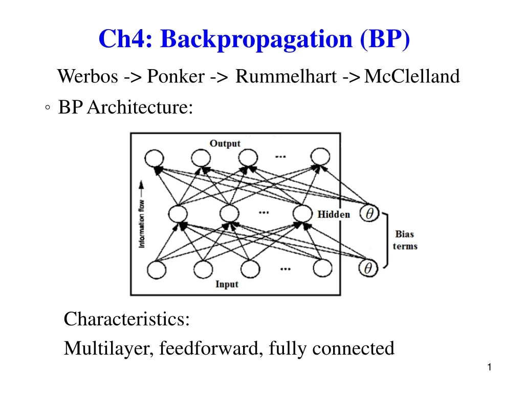
Werbos -> Ponker ->Rummelhart ->McClelland Ch4: Backpropagation (BP) 。BP Architecture: Characteristics: Multilayer, feedforward, fully connected
。 Potential problems being solved by BP 1. Data translation, e.g., data compression 2. Best guess , e.g., pattern recognition, classification Example: Character recognition application a) Traditional method: Translate a 7 × 5 image to 2–byte ASCII code
Lookup table Suffer from: a. Noise, distortion, incomplete b. Time consuming
b) Recent method: Recognition-by-components Traditional approach Neural approach
4.1. BP Neural Network During training, self-organization of nodes on the intermediate layers s.t. different nodes recognize different features or their relationships. Noisy and incomplete patterns can thus be handled.
4.1.2. BP NN Learning Given training examples: , where find an approximation of through learning
4.2. Generalized Delta Rule (GDR) Consider input vector Hidden layer: Net input to the jth hidden unit hidden layer jth hidden unit bias term with jth unit ith input unit Output of the jth hidden unit transfer function
Output layer: 。 Update of output layer weights The error at a single output unit k, The error to be minimized: where M: # output units
The descent direction The learning rule: where: learning rate
。 Determine where L: # hidden units 11
The weights on the output layer are updated as 。 Consider Two forms for the output functions i) Linear ii) Sigmoid or 12
For linear function (A) For sigmoid function Let (A) 14
。 Example 1: Quadratic neurons for output nodes Output function: Sigmoid Determine the updating equations of for output-layer neurons. 15
◎ Updates of hidden-layer weights Difficulty: Unknown outputs of the hidden-layer units Idea: Relate error E to the output of the hidden layer 16
※ The known error (or loss) on the output layer are propagated back to a hidden layer of interest to determine the weight changes on that layer
4.3. Practical Considerations 。 Principles of determining network size: i) Use as few nodes as possible. If the NN fails to converge to a solution, it may need more nodes. ii) Prune the hidden nodes whose weights change very little during training 。 Principles of choosing training data i) Cover the entire domain (representative) ii) Use as many data as possible (capacity) iii) Adding noise to the input vectors (generalization)
。 Parameters: i) Initialize weights with small random values ii) Learning rate η decreases with # iterations η large perturbation η small slow; iii) Momentum technique -- Adding a fraction of the preview change, while tends to keep the weight changes going in the same direction to the weight change, iv) Perturbation – Repeat training using multiple initial weights.
4.4. Applications • Dimensionality reduction: A BPN can be trained to map a set of patterns from an n-D space to an m-D space (m < n).
Data compression - video images The hidden layer represents the compressed form of the data. The output layer represents the reconstructed form of the data. Each image vector will be used as both the input and the target output.
‧ Size: NTSC: National Television Standard Code 525 × 640 = 336000 #pixels/image ‧ Strategy: Divide images into blocks, e.g., 8 × 8 = 64 pixels, 64-output layer, 16-hidden layer, 64-input layer, #nodes = 144
◎ Paint quality inspection Reflects a laser beam off the painted panel and onto a screen Poor paint: Reflected laser beam diffused ripples, orange peel, lacks shine Good paint: Relatively smooth and bright luster Closely uniform throughout its image
The output was to be a numerical score (1(best) -- 20(worst))