Download
1 / 51
530 likes | 616 Vues
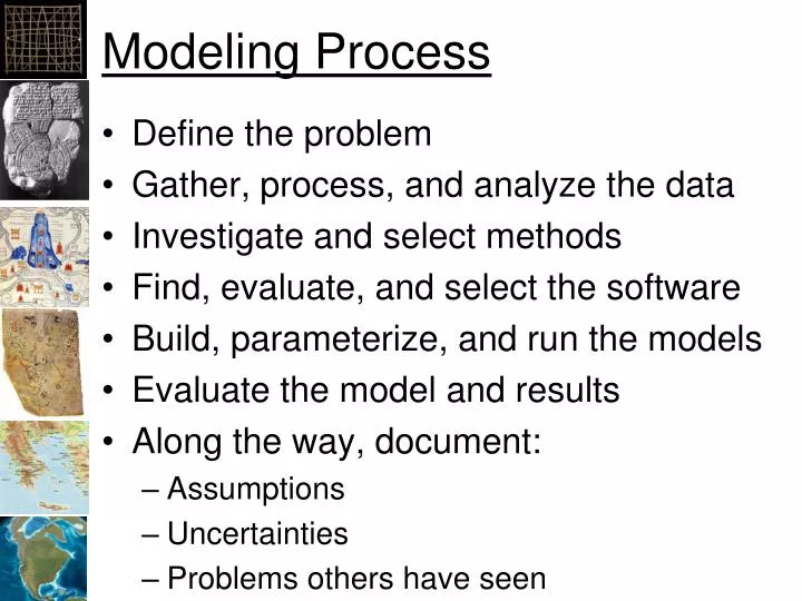
Modeling Process. Define the problem Gather, process, and analyze the data Investigate and select methods Find, evaluate, and select the software Build, parameterize, and run the models Evaluate the model and results Along the way, document: Assumptions Uncertainties

E N D
Modeling Process • Define the problem • Gather, process, and analyze the data • Investigate and select methods • Find, evaluate, and select the software • Build, parameterize, and run the models • Evaluate the model and results • Along the way, document: • Assumptions • Uncertainties • Problems others have seen
Correlation Modeling • Find a “Response” between independent and dependent variables • Environmental Modeling • Finding a response between environmental variables and a species distribution • Habitat Suitability Maps • Species Distribution Maps
Correlation Modeling • Creates a model in N-Dimensional “Hyper-Space” • Vary by: • Mathematics used to create the model • Statistics used to optimize parameters • Options for model evaluation
Habitat Suitability Models • Find the suitable habitat for a species • Also called “Species Distribution Models” Tamarisk, NIISS.org Tree Sparrow, Herts Bird Club
Two Approaches Occurrence/Presence Mechanistic Occurrences “Greenhouse” experiments Correlate Design Model Model Environmental Layers Generate Generate Map
From the Theory of Biogeography + 0 - Salinity Environmental Space Population Growth Niche + 0 - Salinity Temperature Temperature Brown, J.H., Lomolino, M.V. 1998, Biogeography: Second Edition. Sinauer Associates, Sinauer Massachusetts
Early Approaches • BioClim • BioMapper • Genetic Algorithm for Rule Set Production (GARP) • Generalized Linear Models (GLM) • Generalized Additive Models (GAMs) • Kernel Methods • Neural Networks
Latest Approaches • Multivariate adaptive regression splines (MARS) • Maxent – piece-wise regression with Maximum entropy optimization • Hyper-Envelope Modeling Interface (HEMI), Bezier curves • Non-Parametric Multiplicative Regression (NPMR)
Tree Methods • Regression Trees • Boosted Regression Trees • Random Forests
Predicting Habitat Suitability • Predicting potential species distributions at large spatial and temporal extents • Given: • Limited data • Most have unknown uncertainty • Most biased/not randomly sampled • >90% just “occurrences” or “observations” • Lots of species • Climate change and other scenarios
Tree Sparrow Occurrences House Sparrows Eurasian Tree Sparrows Graham, J., C. Jarnevich, N. Young, G. Newman, T. Stohlgren, How will climate change affect the potential distribution of Eurasian Tree Sparrows (Passer montanus)? Current Zoology, 2011.
Modeling Process 100 0 Spreadsheets Occurrences Environmental Layers Temperature Precipitation Modeling Algorithm Model Parameters Habitat Suitability Map Map Generation Habitat Suitability Map for Purple Loostrife by Catherine Jarnevich
Tree Sparrow Model - 2050 Graham, J., C. Jarnevich, N. Young, G. Newman, T. Stohlgren, How will climate change affect the potential distribution of Eurasian Tree Sparrows (Passer montanus)? Current Zoology, 2011
Spatial Modeling Concerns • Over fitting the data • Are we modeling biological/ecological theory? • What does the model look like? • In environmental space vs. geographic space • Absence points? • What do they mean? • Analysis and representation of uncertainty? • Can we really model the potential distribution of a species from a sub-sample?
Occurrences of Polar Bears From The Global Biodiversity Information Facility (www.gbif.org, 2011)
Uncertainty in Data • Experts more accurate in correctly identifying species than volunteers • 88% vs. 72% • Volunteers: 28% false negative identifications and 1% false positive identifications • Experts: 12% false negative identifications and <1% false positive identifications • Conspicuous vs. Inconspicuous • Volunteers correctly identified “easy” species 82% of the time vs. 65% for “difficult” species • 62% of false ids for GB were CB
Geographical Space Observed Occurrences Realized Niche/Distribution Environmental Space Fundamental Niche/Distribution Model Fitted to Occurrences Adapted from Richard Pearson, Center for Biodiversity and Conservation at the American Museum of Natural History
From the Theory of Biogeography + 0 - Salinity Environmental Space Population Growth Niche + 0 - Salinity Temperature Temperature Brown, J.H., Lomolino, M.V. 1998, Biogeography: Second Edition. Sinauer Associates, Sinauer Massachusetts
Germination Percentage Shrestha, A., E. S. Roman, A. G. Thomas, and C. J. Swanton. 1999. Modeling germination and shoot-radicle elongation of Ambrosia artemisiifolia. Weed Science 47:557-562.
Over-fitting The Data? Maxent model for Tamarix in the US: response to temperature when modeled with temperature and precipitation What should the model look like? Maraghni, M., M. Gorai, and M. Neffati. 2010. Seed germination at different temperatures and water stress levels, and seedling emergence from different depths of Ziziphus lotus. South African Journal of Botany 76:453-459.
Maxent Model Parameters • bio12_annual_percip_CONUS, -4.946359908378759, 52.0, 3269.0 • bio1_annual_mean_temp_CONUS, 0.0, -27.0, 255.0 • bio1_annual_mean_temp_CONUS^2, -0.268525818823649, 0.0, 65025.0 • bio12_annual_percip_CONUS*bio1_annual_mean_temp_CONUS, 7.996877654196997, -15579.0, 364506.0 • (681.5<bio12_annual_percip_CONUS), -0.27425992202014554, 0.0, 1.0 • (760.5<bio12_annual_percip_CONUS), -0.0936978541445044, 0.0, 1.0 • (764.5<bio12_annual_percip_CONUS), -0.34195651409710226, 0.0, 1.0 • (663.5<bio12_annual_percip_CONUS), -0.002670474531339423, 0.0, 1.0 • (654.5<bio12_annual_percip_CONUS), -0.06854638847398926, 0.0, 1.0 • (789.5<bio12_annual_percip_CONUS), -0.1911885535421742, 0.0, 1.0 • (415.5<bio12_annual_percip_CONUS), -0.03324755386105751, 0.0, 1.0 • (811.5<bio12_annual_percip_CONUS), -0.5796722427924351, 0.0, 1.0 • (69.5<bio1_annual_mean_temp_CONUS), 0.35186971641045406, 0.0, 1.0 • (433.5<bio12_annual_percip_CONUS), -0.4931182020218725, 0.0, 1.0 • (933.5<bio12_annual_percip_CONUS), -0.6964667980858589, 0.0, 1.0 • (87.5<bio1_annual_mean_temp_CONUS), 0.026976617714580643, 0.0, 1.0 • (41.5<bio1_annual_mean_temp_CONUS), 0.16829480000216024, 0.0, 1.0 • (177.5<bio1_annual_mean_temp_CONUS), -0.10871555671575972, 0.0, 1.0 • (91.5<bio1_annual_mean_temp_CONUS), 0.146912383178006, 0.0, 1.0 • (1034.5<bio12_annual_percip_CONUS), -2.6396398836001156, 0.0, 1.0 • (319.5<bio12_annual_percip_CONUS), -0.061284542503119606, 0.0, 1.0 • (175.5<bio1_annual_mean_temp_CONUS), -0.2618197321200044, 0.0, 1.0 • (233.5<bio1_annual_mean_temp_CONUS), -0.9238257709966757, 0.0, 1.0 • (37.5<bio1_annual_mean_temp_CONUS), 0.3765193693625046, 0.0, 1.0 • (103.5<bio1_annual_mean_temp_CONUS), 0.09930300882047771, 0.0, 1.0 • (301.5<bio12_annual_percip_CONUS), -0.1180307164256701, 0.0, 1.0 • (173.5<bio1_annual_mean_temp_CONUS), -0.10021086459501297, 0.0, 1.0 • (866.5<bio12_annual_percip_CONUS), -0.26959719615289196, 0.0, 1.0 • (180.5<bio1_annual_mean_temp_CONUS), -0.04867293241613234, 0.0, 1.0 • (393.5<bio12_annual_percip_CONUS), -0.11059348100482837, 0.0, 1.0 • (159.5<bio1_annual_mean_temp_CONUS), -0.017616972634255934, 0.0, 1.0 • (36.5<bio1_annual_mean_temp_CONUS), 0.060674971087442194, 0.0, 1.0 • (188.5<bio1_annual_mean_temp_CONUS), -0.03354825843486451, 0.0, 1.0 • (105.5<bio1_annual_mean_temp_CONUS), 0.06125114176950926, 0.0, 1.0 • (153.5<bio1_annual_mean_temp_CONUS), -0.12297221415244217, 0.0, 1.0 • (1001.5<bio12_annual_percip_CONUS), -0.45251593589861716, 0.0, 1.0 • (74.5<bio1_annual_mean_temp_CONUS), 0.026393316564235686, 0.0, 1.0 • (109.5<bio1_annual_mean_temp_CONUS), 0.14526936669793344, 0.0, 1.0 • (105.0<bio12_annual_percip_CONUS), -0.42488171108453276, 0.0, 1.0 • (25.5<bio1_annual_mean_temp_CONUS), 0.003117221628224885, 0.0, 1.0 • (60.5<bio12_annual_percip_CONUS), 0.5069564460069241, 0.0, 1.0 • (231.5<bio12_annual_percip_CONUS), -0.08870602107253492, 0.0, 1.0 • (58.5<bio1_annual_mean_temp_CONUS), -0.23241170568516853, 0.0, 1.0 • (49.5<bio1_annual_mean_temp_CONUS), 0.026096163653731276, 0.0, 1.0 • (845.5<bio12_annual_percip_CONUS), -0.24789751889995176, 0.0, 1.0 • 'bio1_annual_mean_temp_CONUS, -6.9884695411343865, 232.5, 255.0 • (320.5<bio12_annual_percip_CONUS), -0.10845844949785532, 0.0, 1.0 • (121.5<bio1_annual_mean_temp_CONUS), -0.12078290084760739, 0.0, 1.0 • (643.5<bio12_annual_percip_CONUS), -0.18583722923085083, 0.0, 1.0 • (232.5<bio1_annual_mean_temp_CONUS), -0.49532279859757916, 0.0, 1.0 • (77.5<bio12_annual_percip_CONUS), 0.09971599046855084, 0.0, 1.0 • (130.5<bio1_annual_mean_temp_CONUS), -0.01184619743061956, 0.0, 1.0 • (981.5<bio12_annual_percip_CONUS), -0.29393286794072015, 0.0, 1.0 • `bio12_annual_percip_CONUS, 0.023135559662549977, 52.0, 147.5 • 'bio1_annual_mean_temp_CONUS, 1.0069995641400011, 216.5, 255.0 • `bio1_annual_mean_temp_CONUS, 0.9362466512437257, -27.0, 16.5 • (397.5<bio12_annual_percip_CONUS), -0.02296169875555788, 0.0, 1.0 • `bio12_annual_percip_CONUS, 0.14294702222037983, 52.0, 251.5 • (174.5<bio1_annual_mean_temp_CONUS), -0.01232159395283821, 0.0, 1.0 • 'bio1_annual_mean_temp_CONUS, -1.011329703865716, 150.5, 255.0 • `bio12_annual_percip_CONUS, 0.12595056977305263, 52.0, 326.5 • 'bio1_annual_mean_temp_CONUS, -0.6476124017711095, 119.5, 255.0 • 'bio1_annual_mean_temp_CONUS, 1.737841121141096, 219.5, 255.0 • (90.5<bio1_annual_mean_temp_CONUS), 0.012061755141948361, 0.0, 1.0 • `bio12_annual_percip_CONUS, 0.1002190195916142, 52.0, 329.5 • `bio12_annual_percip_CONUS, 0.3321425790853447, 52.0, 146.5 • `bio12_annual_percip_CONUS, -0.3041756531549861, 52.0, 59.0 • (385.5<bio12_annual_percip_CONUS), -0.0014858371668052357, 0.0, 1.0 • (645.5<bio12_annual_percip_CONUS), -0.02553082983087001, 0.0, 1.0 • 'bio12_annual_percip_CONUS, -4.091264412509243, 532.5, 3269.0 • `bio1_annual_mean_temp_CONUS, -0.35523981011398936, -27.0, 111.5 • `bio1_annual_mean_temp_CONUS, -0.21070138315106224, -27.0, 112.5 • `bio1_annual_mean_temp_CONUS, 0.22680342516229093, -27.0, 18.5 • (13.5<bio1_annual_mean_temp_CONUS), -0.04258692136695379, 0.0, 1.0 • `bio1_annual_mean_temp_CONUS, 0.12827234634968193, -27.0, 19.5 • linearPredictorNormalizer, 2.2050375426546283 • densityNormalizer, 1311.2581836276431 • numBackgroundPoints, 10000 • entropy, 8.358957722359722 162 Parameters Maxent model from Tamarix model of western US using precipitation and temperature.
Geographical Space Observed Occurrences Realized Niche/Distribution Environmental Space Fundamental Niche/Distribution Model Fitted to Occurrences Adapted from Richard Pearson, Center for Biodiversity and Conservation at the American Museum of Natural History
Tamarisk Occurrences United States Environmental Space
Some Caveats • We are modeling “observations” • Modeling occurrences with some uncertainty • Modeling the realized niche if the data is a complete sample for the environmental space the species currently occupies • Modeling the fundamental niche if B is true and the species is covering it’s full possible range of habitats • Habitat Suitability Modeling • Predicting the potential species distribution
Problems with Polynomials • Lack flexibility • Not well behaved at boundaries f(x) = a0 + a1x + a2x2 + ... + anxn , where an ≠ 0 and n ≥ 2 Wikipedia.com
Alternatives to Polynomials • BioClim – max and max boxes • BioMapper – 25x25 grid of boxes • DOMAIN – Distance to existing point • NPMR • Hyper-Envelope Modeling – Bezier Curves • Multivariate adaptive regression splines
Bezier and Spline Curves P1 P0 P2 P3 Wikiepedia.com
Modified Bezier Curves S3 S2 P2 P3 S1 P0 P1 S0 International Biological Information Science
“Good” Model Cold Hot
“Poor” Model Cold Hot
Receiver Operator Curve • Model Goal: • Predicts “positive” results “inside” the model • Predicts “negative” results “outside” the model • For a given threshold: • What is the relationship between: • Proportion of positive results within the model • Proportion of negative results outside the model
Receiver Operator Curve Threshold Cold Hot
Area Under the Curve Metric • Area Under the Curve (AUC) • 1=Perfect • 0=Worthless Threshold 1 -> 0
AUC • Metric of “how good” the model is • Does not require a pdf • Can be computed with or without negative results (absences) • Does not include the number of parameters
Tamarisk Occurrences United States Environmental Space
HEMI Tamarix Model 107 AUC: 0.76 Min Temp of coldest Month (°C*10) Potential Habitat 5 Points -> 10 Parameters -231 Unsuitable Habitat 46 3385 Annual Precipitation (mm) International Biological Information Science
Potential Habitat Potential Habitat Unsuitable Habitat International Biological Information Science
Global Tamarisk Map? 1.0 Habitat Suitability International Biological Information Science 2.0
Document Caveats • Assumptions • No errors in the data collection, handling, processing • No software defects • Occurrences represent viable populations in the wild • Density of occurrences correlates with potential habitat • Uncertainties • Field data, environmental layers • 256x256 grid used for 2d histograms
Migration Animations • Jim’s web site • http://tinyurl.com/6krghts • Gray whale model • http://tinyurl.com/4xtmzho • Barn swallows