Download
1 / 37
370 likes | 434 Vues
Simulating Earthquake Ground Motion with the AWM Finite Difference Code. Yifeng Cui, SDSC

E N D
Simulating Earthquake Ground Motion with the AWM Finite Difference Code Yifeng Cui, SDSC In collaboration with Kim Olsen, Philip Maechling, Steve Day, Bernard Minster and Thomas Jordan of the Southern California Earthquake Center, Reagan Moore and Amit Chourasia of San Diego Supercomputer Center
Southern California: a Natural Laboratory for Understanding Seismic Hazard and Managing Risk • Tectonic diversity • Complex fault network • High seismic activity • Excellent geologicexposure • Rich data sources • Large urban population with densely built environment high risk • Extensive research program coordinated by Southern California Earthquake Center under NSF and USGS sponsorship
Major Earthquakes on the San Andreas Fault, 1680-present How dangerous is the San Andreas fault? • The southernmost San Andreas fault has a high probability of rupturing in a large (>M 7.5) earthquake during the next two decades. • Historic earthquakes: • 1906, enormous damage to SF • 1857, 360km long rupture • Major events have not been seen on San Bernardino Mountains • 1994 Northridge • When: 17 Jan 1994 • Where: San Fernando Valley • Damage: $20 billion • Deaths: 57 • Injured: >9000 1906 M 7.8 1680 M 7.7 1857 M 7.9 segment since 1812 and on Coachella Valley segment since ~1680. Average recurrence intervals on these segments are ~150 and ~220 years, respectively.
TeraShake Platform • 600km x 300km x 80km • Spatial resolution = 200m • Mesh Dimensions • 3000 x 1500 x 400 = 1.8 billion mesh points • Simulated time = 3 minutes • Number of time steps = 22,728 (0.011 sec time step) • 60 sec source duration from Denali
AWM Finite Difference Code • Structured 3D with 4th order staggered-grid finite differences for velocity and stress developed by Olsen at UCSB/SDSU • Perfected Matched Layers absorbing boundary conditions on the side and bottom of the grid, zero-stress free surface condition at the top • Fortran 90, massage passing done with MPI using domain decomposition, I/O using MPI-IO • Point-to-point and collective communication • Extensively validated for a wide range of problems
Parallelization strategy • Illustration of the communication between neighboring subgrids over 8 procs • Each processor responsible for performing stress and velocity calculations for its portion of the grid, as well as dealing with boundary conditions at the external edges of each volume. • Ghost cells: two-point-thick padding layer - the most recently updated wavefield parameters exchanged from the edge of the neighboring sub-grid.
Enabling TeraShake on TeraGrid • Challenges for porting and optimization • Challenges for initialization • Challenges for execution • Challenges for data archival and management • Challenges for analysis of results
Challenges for Porting and Optimization • Enhanced from 32-bit to 64-bit for managing 1.8 billion mesh points • Single CPU optimization • Profiling the execution time, identified MPI and MPI-IO bottlenecks • Improved cache performance and interprocedural analysis • Incorporated physically-based dynamic rupture component to simulation to create realistic source description • MPI-IO • Data-Intensive: separate surface from volume • Computing-intensive: accumulate output data in memory buffer until reaching optimized size before writing output to disk • Performance: MPI-IO change from using individual file pointer to using an explicit offset to improve I/O performance • Portability: selection of datatype that represents countblocks with or without stride in terms of defining type
Before SDSC SAC involved Code deals up to 24 million mesh nodes Code scales up to 512 processors Ran on local clusters only No checkpoints/restart capability Wave propagation simulation only Researcher’s own code Large memory needs, not scalable Initialization slow I/O not scalable, slow After SDSC SAC efforts Codes enhanced to deal with 32 billion mesh nodes Excellent speed-up to 40,960 processors, 6.1 Tflop/s Ported to p655, BG/L, IA-64, XT3, Dell Linux etc Added Checkpoints/restart/checksum capability Integrated dynamic rupture + wave propagation as one Serve as SCEC Community Velocity Model Separate mesh partition from solver, scalable 10x speed-up of initialization MPI-I/O improved 10x, scaled up to 40k processors SDSC SAC TeraShake Efforts
Challenges for Initialization • AWM doesn’t separate mesh generator from solver -> prepare source and media partition in advance • Memory required far beyond the limit of the processor -> read source data in bulk • Media input: reading from single line -> in block
13.2G 13.2G 970K Index 13.2G 13.2G 13.2G 13.2G 13.2G Input Input 55M pmap 55M pmap 55M pmap 55M pmap 55M 55M 55M 55M 55M 55M 55M 55M Memory Optimization: Source Memory Allocation: 13.2G vs. 110M !
Challenges for Execution • Large scale simulations expected to take multiple days to complete. -> checkpoints and restart capability • Post-processing visualization -> separate surface and volume outputs with a setting choice • Dealing with large dataset and 10^-14 bit-error-rate -> add parallelized MD5 checksum, for each mesh sub-array in core memory
Challenges for Execution • Memory-intensive: Pre-processing and pos-processing require large memory -> p690 • Computing-intensive: Dynamic simulations need large processors -> NCSA IA-64 • Data-intensive: Wave propagation runs with full volume outputs -> p655 • Extreme-computing: BG/L
Okaya 200m Media Initial 200m Stress modify TeraShake-2 Executions TS2.dyn.200m 30x 256 procs, 12 hrs, Initial 100m Stress modify SDSC IA-64 TG IA-64 GPFS Okaya 100m Media TS2.dyn.100m 10x 1024 procs, 35 hrs TG IA-64 GPFS-wan NCSA IA-64 GPFS NCSA-SAN Network 100m Reformatting 100m Transform 100m Filtering 200m moment rate SDSC-SAN Datastar GPFS TS2.wav.200m 3x 1024 procs, 35 hrs Datastar p690 Velocity mag. & cum peak Displace. mag & cum peak Seismograms Datastar p655 HPSS SRB SAM-QFS Visualization Analysis Registered to Digital Library
Challenges for Data Archive and Management • Run-time data transfer to SAM-QFS and HPSS, moving it fast enough at rate 120MB/s to keep up with 10 TBs/d output • 90k – 120k files per simulation, organized as a separate sub-collection in SRB • Sub-collections published through SCEC digital library • Services integrated through SCEC portal into seismic-oriented interaction environments
Challenges for Analysis of Results • SDSC’s volume rendering tool Vista, based on Scalable Visualization Toolkit, was used for visualizations. • Vista employs ray casting for performing volumetric rendering • Visualizations alone have consumed more than 40k SUs, utilizing 8-256 processors in a distributed manner. • 130k images in total • Web Portal uses LAMP (Linux, Apache, MySQL, PHP) and Java technology for web middle-waret
-1 Kinematic Source Description
Source and 3D Velocity Model Characterization SCEC Community Velocity Model (CVM) V.3.0
TeraShake-1 Conclusions • NW-directed rupture on southern San Andreas Fault is highly efficient in exciting L.A. Basin • Maximum amplification from focusing associated with waveguide contraction • Peak ground velocities exceeding 100 cm/s over much of the LA basin • Uncertainties related to simplistic source description: • TeraShake 2 …
-2 Spontaneous Rupture Description
TeraShake-2 Overview Preparation of Crustal Model Used for Dynamic Rupture Propagation: 5 sub-volumes with planar fault segments extracted and stitched together to generate volume with a single planar fault segment Some smoothing of velocity model required at stitching points • Rupture dynamic propagation • 1446x400x200 mesh for 200m • 2992x800x400 mesh for 100m • Wave propagation • 3000x1500x400 mesh Fault 80km N 40km 50km 200km 50km
TeraShake-2 Conclusions • Extremely nonlinear dynamic rupture propagation • Effect of 3D velocity structure: SE-NW and NW-SE dynamic models NOT interchangeable • Stress/strength/tapering - weak layer required in upper ~2km to avoid super-shear rupture velocity • Dynamic ground motions: kinematic pattern persists in dynamic results, but peak motions 50-70% smaller than the kinematic values due to less coherent rupture front
TeraShake 1.3 PGV Cumulative Peak Velocity Magnitude
TeraShake 2.1 PGV Cumulative Peak Velocity Magnitude
Porting to BG/L • MPI-IO compiler patches • Code optimization to BG/L • Reduce memory requirements • Reduce initialization time needed • Convert from 64-bit back to 32-bit • Prepare PetaShake 0.75 Hz 150-m run • Separate source and media partition from solver, prepare 40,960 input files in advance • Compilation on BG/L • -O4 adds compile-time inter-procedural analysis • VN mode used for AWM • good use of gpfs-wan to avoid memory limitation
AWM PetaShake Benchmark SimulationsRun on BGW A breakthrough in the field of earthquake ground motion simulation • 800km x 400km x 100km (V4) • Spatial resolution = 100 m • 32 billion mesh points • Min. S wave velocity = 500 m/s • Simulated time = 1 sec • Time steps = 101 • Single point source Seismic hazard map of Southern California, showing four proposed regions for PetaSHA simulations: Northridge domain (V1), PSHA site volume (V2), regional M 7.7 domain (V3), and regional M 8.1 domain (V4)
AWM Code Achieves Excellent Strong Scaling to 40K Cores on BGW • AWM scaled to regional M 8.1 domain with 32 billion mesh points (outer/inner scaling ratio of 8,000) • Parallel efficiency of 96% on 40K BGW cores • Performance achieved 6.1 Teraflop/s on BGW
AWM Code Achieved Excellent Weak Scaling to 32K Cores on BGW • Two problem domains considered Grid at 0.4 km 0.2 km 0.13 km 0.1 km 0.2 km 0.1 km 0.07 km 0.05 km
BG/L Interconnection Networks 3 Dimensional Torus • Interconnects all compute nodes (65,536) • Virtual cut-through hardware routing • 1.4Gb/s on all 12 node links (2.1 GB/s per node) • 1 µs latency between nearest neighbors, 5 µs to the farthest • 4 µs latency for one hop with MPI, 10 µs to the farthest • Communications backbone for computations • 0.7/1.4 TB/s bisection bandwidth, 68TB/s total bandwidth Global Tree • One-to-all broadcast functionality • Reduction operations functionality • 2.8 Gb/s of bandwidth per link • Latency of one way tree traversal 2.5 µs • ~23TB/s total binary tree bandwidth (64k machine) • Interconnects all compute and I/O nodes (1024) Ethernet • Incorporated into every node ASIC • Active in the I/O nodes (1:64) • All external comm. (file I/O, control, user interaction, etc.) Low Latency Global Barrier and Interrupt • Latency of round trip 1.3 µs Control Network
Moving from TeraShake to PetaShake • PetaShake as SCEC’s advanced platform for petascale simulations of dynamic ruptures and ground motions with outer/inner scale ratios as high as 104.5 • TeraShake outer/inner scale ratio of 103.5
Summary • TeraShake demonstrated that optimization and enhancement of major applications codes are essential for using large resources (number of CPUs, number of CPU-hours, TBs of data produced) • TeraShake showed that multiple types of resources are needed for large problems: initialization, run-time execution, analysis resources, and long-term collection management • TeraShake code as a community code now used by the wide SCEC community • Significant TeraGrid allocations are required to advance the seismic hazard analysis to a more accurate level • Next: PetaShake!
Acknowledgements • SCEC: Kim Olsen, Bernard Minster, Steve Day, Luis Angel Dalguer, David Okaya, Phil Maechling and Thomas Jordan • SDSC: Dong Ju Choi, Layton Chen, Amit Chourasia, Steve Cutchin, Larry Diegel, Nancy Wilkins-Diehr, Marcio Faerman, Robert Harkness, Yuanfang Hu, Christopher Jordan, Tim Kaiser, George Kremenek, Yi Li, Jon Meyer, Amit Majumdar, Reagan Moore, Richard Moore, Krishna Muriki, Arcot Rajasekar, Donald Thorp, Mahidhar Tatineni, Paul Tooby, Michael Wan, Brian John White, Tony Vu and Jing Zhu • NCSA: Jim Glasgow, Dan Lapine • IBM TJ Watson: Fred Mintzer, Bob Walkup, Dave Singer • Computing resources are from SDSC, NCSA, PSC, IBM TJ Watson. • SDSC's computational collaboration effort was partly supported through the NSF-funded SDSC Strategic Applications Collaborations (SAC) programs, and through TeraGrid ASTA. SDSC Visualization effort was supported through SDSC core program. SCEC Community Modeling Environment is funded through NSF ITR/GEO grants.