Download
1 / 19
190 likes | 315 Vues
Status of Reference Network Simulations. John Dale ILC-CLIC LET Beam Dynamics Workshop 23 June 2009. Introduction. Alignment Concept Summary Of Previous Talks Linear model Free network solution Problems with model Too simple Generation of constraints Solutions to Problems

E N D
Status of Reference Network Simulations John Dale ILC-CLIC LET Beam Dynamics Workshop 23 June 2009
Introduction • Alignment Concept • Summary Of Previous Talks • Linear model • Free network solution • Problems with model • Too simple • Generation of constraints • Solutions to Problems • 4 marker network • EVD to determine eigenvectors • Updated model comparison with panda • Future Work
X Z Accelerator Alignment Concept Accelerator • Many possible ways to Align an Accelerator, the concept used here is: • Over lapping measurements of a network of reference markers using a device such as a laser tracker or a LiCAS RTRS • Measurements of a small number of Primary Reference Markers (PRM) using, for example GPS transferred from the surface. • Combining all measurements in a linearised mathematical model to determine network marker positions • Using adjusted network to align Main Linac • Using Dispersion Matched Steering (DMS) to adjust correctors to minimise emittance PRM Reference Marker Machine Marker Stake out device
Reference Network Simulation Aims • Generate ILC reference network solutions which can be used for LET simulations • Easy to use • Quickly (minutes not days) • Correct statistical properties • Capable of simulating existing as well as novel network measurement techniques
Possible Approaches • Commercial survey adjustment software • Expensive • Need to be survey expert to use • Usually only use laser tracker/tachometers • Full simulation of a specific device • Slow to generate networks • Restricted to one measurement technique • Simplified Model • If designed correctly can be quick • Can be used to model novel devices
Simplified Model • Have a device model • measures small number of RMs e.g. 4 • moves on one RM each stop and repeats measurement • rotates around the X and Y axis • determines vector difference between RMs • only the error on the vector difference determination is required as input • PRM measurements are vector difference measurements between PRM’s
The Linearised Model • M device stops, N reference Markers Total, O PRMs Total, device measures 4 markers per stop • Measurement Vector L • Contains device and PRM vector differences • Measurement Covariance Matrix P • Simple diagonal matrix assuming no cross dependency on measurements • Variables Vector X • Contains all the markers positions • Prediction Vector F(X) • Predicts L • Difference Vector W = F(X) – L • Design Matrix A = δF(X)/δX
The Linearised Model • Normal Non-linear least squares minimises WTW leading to an improvement of estimates given by ΔX = -(ATPA)-1ATPW • Problem ATPA is singular and not invertible • Model Requires Constraints.
Free Network Constraints • Five constraints required • Could constrain first point to be at (0,0,0) and both the rotations of first stop to be 0. • Gives zero error at one end and large error at other. Not the desired form • Use a free network constraint • Technique developed in Geodesy • The free network constraint is that XTX is minimised. • If XTX = min the trace of the output covariance matrix is also minimised • Equivalent to a generalised inverse • The least squares minimises WTW and XTX to give a unique solution
Free Network Constraints • In a free network, the least squares solver is of the form • Errors are of the form • Need to determine A2t and A2 • A2t and A2 are the matrix of eigenvectors corresponding to the zero (or small) eigenvalues
Free Network Constraint • Break Up ATPA into sub-matrices • N11 Must be non-singular • N22 size 6*6 • Leading to constraint Matrix A2
Model Summary • Input • Device Measurement Errors • Number RMs measured by device in one stop • PRM Measurement Errors • Network Parameters • Number RMs, Number PRMS, RM spaceing, PRM spacing • Output • Reference marker position difference from truth • Reference marker position statistical error
Laser Tracker Network Simulation • Test model by comparing to laser tracker network • Can simulate ILC laser tracker networks using PANDA • Use PANDA output to determine model parameters • minimising the difference between the PANDA statistical errors and the model statistical errors • Minimiser can adjust the model input parameters • minisation using JMinuit
Problems with previous version • Had model which solved, but error curves didn’t match PANDA
Problems Two problems with model 1) The network was too simple • A single line of points did not give sufficient strength to the network 2) Method of determining eigenvectors • Method used only works for very well behaved matrices
Solutions 1) The network was too simple • Allow more complex 3D networks to be used • Simulations now use four markers in a ring 2) Method of determining eigenvectors • Determine the eigenvectors using more complex methods such as Eigen Value Decomposition (EVD)
Model vs PANDA • Much better match between the PANDA and Model error curves
Model Status • How to determine constraints better understood • Determination of constraints is slow, especially on the full networks • EVD generates all eigenvalues and eigenvectors • One eigenvalue for each element in the network • 40 minutes for a single iteration • Many iterations required for solution
Future Work • Determine required eigenvectors faster • Only require 6 eigenvectors, corresponding to the small eigenvalues. • Test updated model with DMS simulations • Distribute code