Download
1 / 12
140 likes | 356 Vues
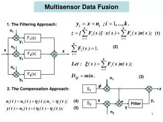
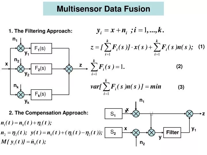
n 1. F 1 (s). y 1. n 2. x. z. F 2 (s). y 2. n k. F k (s). n 1. y k. x. x. z. S 1. x. y 1. S 2. Filter. y. n 2. 1. The Filtering Approach:. (1). Multisensor Data Fusion. (2). (3). 2. The Compensation Approach:. n. y. e. W(s). F(s). x. I(s)=1.

E N D
n1 F1(s) y1 n2 x z F2(s) y2 nk Fk(s) n1 yk x x z S1 x y1 S2 Filter y n2 1. The Filtering Approach: (1) Multisensor Data Fusion (2) (3) 2. The Compensation Approach:
n y e W(s) F(s) x I(s)=1 Optimal Filtration in Scalar Case. (4) (5) Wiener-Hopf Equation: (6) (7)
Wiener Factorization: (8) Wiener Separation: (9) Optimal Filter: (10) Example: (11) (12) (13)
n W(s) F(s) x y n1 z F1(s) W1(s) y1 ε Optimal Fusion of 2 sensors. (1) i (2) (3) (4) (5) (6)
Wiener-Hopf equation: (7) (8) (9) Example: fusion of Doppler and barometric speed sensors: Barometric: (10) (11) Doppler: (12) where:
Discrete Kalman Filter Discrete observed plant: x[n+1] = Anx[n] + w[n]{State equation} y[n] = Cnx[n] + v[n] {Measurements} M{ww'} = Qn, M{vv'} = Rn, M{wv'} = Nn=0, (1) (1a) Performance index: State vector prediction: x[n+1/n] = Anx[n/n]; (2a) Covariance matrix prediction: (2b)
Discrete Observer: Measurement update: X[n+1/n] = AnX[n/n-1] + Kn/n-1 (y[n] - CnX[n/n-1]); X[n/n] = X[n/n-1] + Kn (y[n] - CnX[n/n-1]) Y[n/n] = CnX[n/n]; Pn/n-1 = E{(x[n] - X[n|n-1])(x[n] - X[n|n-1])'} (Ric. solution) Pn/n= E{(x[n] - X[n|n])(x[n] - X[n|n])'} (Updated estimate) Time update: (3) (4) Covariance Matrices: (5) (6) (7)
P(0),X(0),An, Cn,Qn,Rn. Initial data: z-1 z-1 Measurements y[n] X[n/n] = AnX[n/n-1] + Kn (y[n] - CnX[n/n-1]) Time-dependant Kalman Filter Algorithm 1 2 3 4 5 6 7
v1 w1 FK RNS w2 DRS yn/n v2 Example: fusion of the dead reckon and radio-navigation systems
Dec. Bin. Grey 0 0 0 0 0 0 0 y 1 0 0 1 0 0 1 2 0 1 0 0 1 1 x 0 1 3 0 1 1 0 1 0 0 0 1 4 1 0 0 1 1 0 1 1 0 5 1 0 1 1 1 1 6 1 1 0 1 0 1 7 1 1 1 1 0 0 Hd=3 1. Coding of Signals. Hamming’s distance: Grey Code. Example: 3-digit word Transmission of Information Encoding: Truth Table: Decoding:
Com. Ch. LPF CSG ym ym 2. Modulation of Signals