Download
1 / 30
300 likes | 525 Vues
Money in the Competitive Equilibrium Model Part 2. Explicit Money Demand Cash-in-Advance Model Optimal Monetary Policy. Money and Real Ecomomic Variables. Neutrality of Money a one-time change in the level of the nominal money supply has no effect on real economic variables (only nominal).

E N D
Money in the Competitive Equilibrium ModelPart 2 Explicit Money Demand Cash-in-Advance Model Optimal Monetary Policy
Money and Real Ecomomic Variables • Neutrality of Money a one-time change in the level of the nominal money supply has no effect on real economic variables (only nominal). • Superneutrality of Money a change in the growth rate of the money supply has no effect on real economic variables. • Sometimes “superneutrality” definition exclued the real money supply as a “real” economic variable.
CE model with Ad-Hoc money demand (e.g. Cagan model) money is neutral and superneutral. • An increase in the money growth rate • Classical dichotomy No change in CE values of y*,N*,c*, and r*. • This result may not be true in CE model with explicit money demand.
Reminder: Nominal versus Real Interest Rates: (exact) or r = R – p (approx) where R = nominal rate r = real rate inflation rate =
Explicit Money Demand • Incorporate use of money as a decision of the representative household. • Assumptions: (A1) Income yt is exogenous (A2) Households make an asset allocation decision between nominal money (M) and bonds (B). (A3) TO BE ADDED (A4) Government directly sets nominal Ms (A6) No uncertainty
Money Supply: where Xt = transfer of money to public (“helicopter drop”) and m = money growth rate • Reminder: Real vs Nominal Interest Rates: (1+r) = (1+R)/(1+p) or r = R – p (approx) where
Timeline • Budget Constraint (nominal terms) (BC) Total Sources of Income = Total Uses • Optimization: Choose {ct, Mt, Bt} to subject to (BC)
State Variables: Control Variables: • Bellman Equation: subject to (transition equation)
FOC and Envelope conditions contradict unless R = 0. • If R > 0 then M = 0. Money is an inferior asset to bonds and valueless. • Need another constraint to give money value.
Cash-in-Advance Model (A3): Consumption must be purchased with cash carried in advance from previous period. • New Timeline • Cash-In-Advance Constraint (CIA)
State Variables: Control Variables: • Bellman Equation: CIA Constraint subject to
FOC & Envelope (1) • Market-Clearing (MC): Goods: ct = yt = y* Money: Mt = Mts Bonds: Bt = 0 (Note from BC if two of the three markets clear, the third one will also clear)
The CE are values for {ct, yt, Bt, rt, m=(M/P), R, p} solving (1), (2) and (MC) conditions. • CE Values: c* = y* (exogenous) p* = m r* = (1/b – 1) = r (M/P)* = c* (Neutrality) (1+R) = (1+r*)(1+p*) (Fisher Effect)
One time changes in the level of Ms are neutral. • Increases in the growth rate of money (m) leads to an increase in p* and R* while leaving c*, y*, r* unchanged. (Superneutrality) • This result comes from exogenous income and is not general when model is modified. • Consider adding labor market and firms to the model.
Figure 15.4 Scatter Plot of the Inflation Rate vs. the Growth Rate in M0 for the United States, 1960–2003
CIA Model with Production • Cooley and Hansen (1989 – AER) • Modify to Include Labor and Production (1) yt = f(Nt) (2) Utility in each period: U(ct,lt) = u(ct) + u(lt) (3) Firms demand labor to max P = f(N) - wN (4) Modify (BC) (BC) (5) (CIA) is the same
Household FOCs (FOC1) (FOC2)
Firm FOC: (FOC3) • Market-Clearing (MC): Goods: ct = yt Money: Mt = Mts Bonds: Bt = 0 Labor: Nts = Ntd = Nt • Utility: Assume u(c,l) = ln(c) + ln(l)
A steady state equilibrium occurs where N, c, y, (M/P) are constants (to be determined, NOT exogenous):
Steady State CE Values: (s1) p* = m (s2)r* = (1/b – 1) = r (s3) (1+R) = (1+r*)(1+p*) (Fisher Effect) (s4) (s5) c* = y* = f(N*) = (M/P)=m* • Notice (s4) N* and there will be an inverse relationship between N* and m.
In CIA model with production money is neutral but not superneutral. • Money growth and inflation negatively affects employment, consumption, output, real balances. • Inverse Phillips Curve - relation between inflation and “unemployment” is upward sloping. • Inflation “taxes” work and households substitute towards leisure.
Inflation & Employment: Cross Country Study [Cooley & Hansen (1989)] Xass 1976-1985 Austria, Belgium Demark, Finland France, Germany Greece, Ireland, Italy Netherlands, Norway Portgual, Spain Switzerland, UK Canada, US, Australia New Zealand, Japan Chile, Venezuela Vertical Axis = employment
Costs of Inflation and Optimal Monetary Policy • Recall relation between nominal and real interest rates: (approx) (actual) • CEM (in steady state) r* = r constant. • increase mincreases p increases R
High inflation leads to higher costs of conducting transactions with currency (“shoe-leather” costs). • Welfare costs of inflation: Lucas (2000, Econometrica) estimates that reducing US steady inflation from 10% to 0% is equivalent to 1% gain in real GDP. • What is the optimal money growth rate m* in the CE/CIA model with production? • What’s the “optimal” inflation rate in the long-run?
What value of m maximizes utility of the representative household? • The best (welfare maximizing) allocation is the Pareto Optimal allocation: MRSl,c = w MRSct,ct+1 = (1+r*) • Money distorts the optimal decisions of individuals away from social planner.
The “Friedman Rule” says that the optimal monetary policy is to deflate the money supply and prices at a rate which drives R = 0: (i) If R = r* + p , R = 0 m* = p = -r* < 0 (ii) If (1+R) = (1+r)(1+p) = (1+p)/b R = 0 m* = p = b - 1 < 0 • The Friedman Rule requires deflation at the real interest rate or rate of time preference. (M. Friedman – The Optimum Quantity of Money, 1969)
Practical Considerations * Drive the nominal rate on riskless assets (government bonds) to zero. * Nominal variables (wages) are downward rigid. * There are always temptations to inflate the money supply (funding G, business cycles). * Assumes certainty about money/prices. * Most economists agree that low inflation (rather than deflation) is more practical.
Current monetary policy and the Friedman rule: • High money growth rate • Historically Low Nominal Interest Rates • Moderate/Low Inflation • Model provides good description of long-runor steady inflation but lacks “liquidity effects” important for business cycle analysis. • Solution? Modify Model or abandon market-clearing (stick prices, IS-LM?) • Readings: Williamson, Ch 10, p 363-368, 377-388, 395-399 Williamson, Ch 15, p 559-575