INTERNAL FORCED CONVECTION

1. INTERNAL FORCED CONVECTION Nazaruddin Sinaga Laboratorium Efisiensi dan Konservasi Energi

2. Internal Flow The development of the boundary layer for laminar flow in a circular tube is represented in Fig. 17.11. Because of viscous effects, the uniform velocity profile at the entrance will gradually change to a parabolic distribution as the boundary layer begins to fill the tube in the entrance region.

4. Beyond the hydrodynamic entrance length, the velocity profile no longer changes, and we speak of the flow as hydrodynamically fully developed. The extent of the entrance region, as well as the shape of the velocity profile, depends upon Reynolds number, which for internal flow has the form

5. where um is the mean (average) velocity; D, the tube diameter, is the characteristic length; and is the mass flow rate. In a fully developed flow, the critical Reynolds number corresponding to the onset of turbulence is ReD ≈ 2300

6. although much larger Reynolds numbers (ReD≈ 10,000) are needed to achieve fully turbulent conditions. For laminar flow (ReD = 2300), the hydrodynamic entry length has the form (XL/D )lam 0.05 ReD

7. while for turbulent flow, the entry length is approximately independent of Reynolds number and that, as a first approximation 17.40 For the purposes of this text, we shall assume fully developed turbulent flow for (x/D) > 10.

8. If fluid enters the tube at x = 0 with a uniform temperature T(r,0) that is less than the constant tube surface temperature, Ts , convection heat transfer occurs, and a thermal boundary layer begins to develop.

10. In the thermal entrance region, the temperature of the central portion of the flow outside the thermal boundary layer, δt, remains unchanged, but in the boundary layer, the temperature increases sharply to that of the tube surface.

11. At the thermal entrance length, xfd,t, the thermal boundary layer has filled the tube, the fluid at the centerline begins to experience heating, and the thermally fully developed flow condition has been reached. For laminar flow, the thermal entry length may be expressed as

12. From this relation and by comparison of the hydrodynamic and thermal boundary layers of Fig. 17.11a and 17.11b, it is evident that we have represented a fluid with a Pr < 1 (gas), as the hydrodynamic boundary layer has developed more slowly than the thermal boundary layer (xfd,h>xfd,t). For liquids having Pr > 1, the inverse situation would occur.

13. For turbulent flow, conditions are nearly independent of Prandtl number, and to a first approximation the thermal entrance length is

14. The Mean Temperature. The temperature and velocity profiles at a particular location in the flow direction x each depend on radius, r. The mean temperature of the fluid, also referred to as the average or bulk temperature, shown on the figure as Tm(x), is defined in terms of the energy transported by the fluid as it moves past location x.

15. For incompressible flow, with constant specific heat cp, the mean temperature is found from

16. where umis the mean velocity. For a circular tube, dAc = 2πrdr, and it follows that : 17.44

17. The mean temperatureis the fluid reference temperature used for determining the convection heat rate with Newton’s law of cooling and the overall energy balance. Newton’s Law of Cooling. To determine the convective heat flux at the tube surface, Newton’s law of cooling, also referred to as the convection rate equation, is expressed as

18. where h is the local convection coefficient. Depending upon the method of surface heating (cooling), Tscan be a constant or can vary, but the mean temperature will always change in the flow direction. Still, the convection coefficient is a constant for the fully developed conditions we examine next.

19. Fully Developed Conditions. The temperature profile can be conveniently represented as the dimensionless ratio (Ts -T )/(Ts -Tm). While the temperature profile T(r) continues to change with x, the relative shape of the profile given by this temperature ratio is independent of x for fully developed conditions. The requirement for such a condition is mathematically stated as 17.46

20. where Ts is the tube surface temperature, T is the local fluid temperature, and Tmis the mean temperature. Since the temperature ratio is independent of x, the derivative of this ratio with respect to r must also be independent of x.

22. Evaluating this derivative at the tube surface (note that Ts and Tm are constants in sofar as differentiation with respect to r is concerned), we obtain

23. Substituting for from Fourier’s law, is of the form

24. and for q”sfrom Newton’s law of cooling, we obtain

25. Hence, in the thermally fully developed flow of a fluid with constant properties, the local convection coefficient is a constant, independent of x. The last equation is not satisfied in the entrance region where h varies with x.

26. Because the thermal boundary layer thickness is zero at the tube entrance, the coefficient is extremely large near x = 0, and decreases markedly as the boundary layer develops, until the constant value associated with the fully developed conditions is reached.

27. Hydrodynamically fully developed: Thermally fully developed:

29. Energy Balances and Methods of Heating Because the flow in a tube is completely enclosed, an energy balance may be applied to determine the convection heat transfer rate, qconv, in terms of the difference in temperatures at the tube inlet and outlet.

30. From an energy balance applied to a differential control volume in the tube, we will determine how the mean temperature Tm(x) varies in the flow direction with position along the tube for two surface thermal conditions (methods of heating/cooling).

31. Overall Tube Energy Balance. Fluid moves at a constant flow rate and convection heat transfer occurs along the wall surface. Assuming that fluid kinetic and potential energy changes are negligible, there is no shaft work, and regarding cpas constant, the energy rate balance reduces to give

32. where Tmdenotes the mean fluid temperature and the subscripts iand o denote inlet and outlet conditions, respectively. It is important to recognize that this overall energy balance is a general expression that applies irrespective of the nature of the surface thermal or tube flow conditions.

34. Energy Balance on a Differential Control Volume. We can apply the same analysis to a differential control volume within the tube as shown in Fig. 17.14b by writing Eq. 17.48 in differential form 17.49

35. We can express the rate of convection heat transfer to the differential element in terms of the surface heat flux as 17.50 where P is the surface perimeter. Combining Eqs. 17.49 and 17.50, it follows that

36. By rearranging this result, we obtain an expression for the axial variation of Tm in terms of the surface heat flux 17.51

37. or, using Newton’s law of cooling, Eq. 17.45, with q”s=h(Ts - Tm), in terms of the tube wall surface temperature 17.52

38. Thermal Condition: Constant Surface Heat Flux, q”s For constant surface heat flux thermal condition (Fig. 17.15), we first note that it is a simple matter to determine the total heat transfer rate, qconv. Since q”sis independent of x, it follows that 17.53

39. This expression can be used with the overall energy balance, Eq. 17.48, to determine the fluid temperature change, Tm,o-Tm,i. For constant q”s it also follows that the right-hand side of Eq. 17.51 is a constant independent of x. Hence

41. Integrating from x = 0 to some axial position x, we obtain the mean temperature distribution, Tm(x) 17.54

42. Thermal Condition: Constant Surface Temperature, Ts

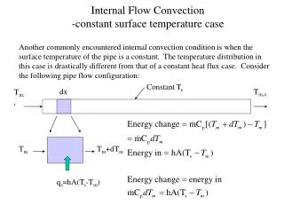
43. Results for the total heat transfer rate and the axial distribution of the mean temperature are entirely different for the constant surface temperature condition (Fig. 17.17). Defining ΔT as (Ts -Tm), Eq. 17.52 may be expressed as

44. With constant, separate variables and integrate from the tube inlet to the outlet

45. From the definition of the average convection heat transfer coefficient, Eq. 17.8, it follows that 17.55a where or simply is the average value of h for the entire tube. Alternatively, taking the exponent of both sides of the equation 17.55b

46. If we had integrated from x = 0 to some axial position, we obtain the mean temperature distribution, Tm(x) 17.56

47. where is now the average value of h from the tube inlet to x. This result tells us that the temperature difference (Ts-Tm) decreases exponentially with distance along the tube axis. The axial surface and mean temperature distributions are therefore as shown in Fig. 17.18.

48. Determination of an expression for the total heat transfer rate qconv is complicated by the exponential nature of the temperature decrease. Expressing Eq. 17.48 in the form and substituting for from Eq. 17.55a, we obtain the convection rate equation 17.57

49. where Asis the tube surface area (As = P.L ) and ΔTlm is the log mean temperature difference (LMTD) 17.58

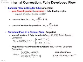
50. Convection Correlations for Tubes: Fully Developed Region To use many of the foregoing results for internal flow, the convection coefficients must be known. In this section we present correlations for estimating the coefficients for fully developed laminar and turbulent flows in circular and noncircular tubes.