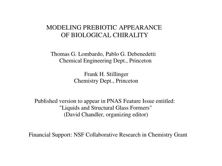
MODELING PRE-BIOTIC APPEARANCE OF BIOLOGICAL CHIRALITY [101st Statistical Mechanics Conference, Rutgers Univ., May 10, 2

2. MODELING PRE-BIOTIC APPEARANCE OF BIOLOGICAL CHIRALITY [101st Statistical Mechanics Conference, Rutgers Univ., May 10, 2009] View 1. Title, collaborators, PNAS issue, NSF support One of the more intriguing challenges presented by molecular biology is why so many of the chemical building blocks out of which living organisms are formed display an almost completely broken symmetry with respect to right and left hand geometries. In other words terrestrial life exhibits a single chirality. As emphasized in View 2 this is evident in observed molecular structures of proteins, DNA, carbohydrates, and other biopolymers.

4. View 2. Motivating mysteries These observations naturally raise basic questions: (a) how did this broken geometric symmetry arise on the early earth, and (b) is the appearance of life and its subsequent evolution contingent on such broken symmetry? It also leads astrobiologists to wonder about the presence of opposite chirality elsewhere in the universe. It may never be possible to attain definitive answers to these questions. However it is feasible to explore possible physical and chemical scenarios that conceivably could have produced the observed broken symmetry. In that spirit the purpose of this short lecture is to propose and describe one model for a possible contributor to the present terrestrial situation. With one exception (glycine) the amino acids serving as the building blocks of proteins individually are chiral. They exhibit only one form in terrestrial biology. The following View 3 illustrates this for the specific case of alanine.

6. View 3. D and L forms of alanine. The rigid tetrahedral bonding at the central carbon atom produces two distinct arrangements of the four attached groups. Biologically occurring alanine, either by itself or as a subunit in proteins, exhibits the so-called "L" form indicated on the left. Not surprisingly this area has a long history of experiment and speculative theory. And not surprisingly it has spawned its own lexicon of chemical jargon. A few of its frequently used symbols, words, and phrases are displayed on View 4.

8. View 4. Some chemical jargon One confusing situation concerns the naming of the enantiomers -- the mirror image molecular twins. Each of the three alternatives has a precise definition, but they use basically different rules. In the case of amino acids whether free or incorporated in proteins the "D,L" convention is the usual choice. The refereed published literature advocates several possible mechanisms for emergence of a dominating chirality. The next View 5 lists five of these.

10. View 5. Possible mechanisms The first entry involving weak interactions has been proposed but is almost certainly orders of magnitude too weak to be a serious contender. My Princeton colleagues and I have generated simple models illustrating scenarios (3) and (4). Limited time here will only allow presenting aspects of (3). In fact our interest in (3) was stimulated by published experiments concerning relevant characteristics of equilibrium phase diagrams for three-component systems. In particular these experiments involved D and L forms of amino acids plus a relatively poor solvent.

12. View 6. Equilateral triangle for 3-component systems; fixed T,p [tutorial.png] For those who might not be familiar with the conventional way that chemists and engineers graphically present those 3-component results View 6 shows the underlying convention based on an equilateral triangle whose vertices represent the pure species. The normal distances to opposite sides from those vertices are proportional to the respective mole fractions. With that background on phase diagram display convention, the following View 7 presents a key experimental result from Imperial College, London published in Nature in 2006.

14. View 7. Phase diagram portion, D,L proline + DMSO; ambient conditions [Fig. 2, Nature article] Because the non-chiral solvent DMSO is a rather poor solvent for the proline enantiomers, only a relevant small portion of the entire 3-component triangle near the pure-DMSO vertex is shown. Four distinct phase (as well as their coexistence regions are shown: dilute liquid solution, pure D-proline and pure L-proline crystals, and a racemic D,L-proline crystal. Of course the diagram has bilateral symmetry about the vertical line passing through the DMSO vertex. The significance of the experimental result is the appearance of the phase boundary maximum ("R") below the solution region, flanked by a pair of off-symmetry eutectic points. This produces a scenario roughly analogous to the familiar case of a zero-field ferromagnetic Ising model cooled reversibly from high temperature through its Curie point, with random small fluctuations steering it either to a fully up or fully down final spin state. The amino acid solution version starts with a virtually racemic very dilute solution very near the upper vertex, followed by solvent evaporation moving the state point downward toward the boundary maximum, then departing left or right to one of the eutectics. Which way it departs depends simply on which random small fluctuation in chiral molecule numbers happened accidentally to be present. Upon reaching the eutectic, the remaining liquid displays a macroscopic EE. The mechanism involves tying up equal numbers of D and L molecules in the racemic crystal. But keep in mind that the boundary maximum is not a solution critical point.

16. View 8. Elementary model, square lattice, 9 site states View 8 indicates how this kind of phase diagram might be approached theoretically using a "minimalist" classical model. It resides on the square lattice in two dimensions. Each site of the lattice can host any one of nine states. Eight of these, shown as bent arrows, represent chiral molecules. The ninth state represents a non-chiral solvent. As shown, the "D" and "L" molecules each have four possible orientations, with their "arms" pointing to nearest-neighbor sites. Solvents are structureless. The enantiomorphs are not interconvertible, they are stable so initial composition remains unchanged. Three short-range interactions are postulated, each negative. The first (v0) acts between any nearest-neighbor pair of chiral molecules regardless of their orientation or chirality; this controls the limited solubility required. The second (v1) is an additional interaction for any nearest neighbor pair of molecules that are identical twins with respect to both chiral character and orientation; this allows for stable pure-enantiomorph crystals when only solvent and one dominating enantiomorph are present. Finally a four-site interaction (v2) arises for any elementary square of sites around which molecules reside with alternating chirality and common orientation of the bent backbones; this allows for existence of a stable racemic crystal.

18. View 9. Formation of crystals at low T (or high concentration); interaction inequality View 9 illustrates the pure-enantiomer and racemic crystal forms. Note that an inequality involving v1 and v2 must be obeyed to ensure stability of the latter. Unfortunately no analytical method is available for exactly solving this nine-state two-dimensional model. We have relied on the well-known but obviously approximate mean-field approach, as outlined on View 10.

20. View 10. Free energy and phase diagram estimation Mean-field approximations are unreliable when critical points are involved, but that is not the case here. We believe that approximation preserves the qualitative nature of the phase diagram for the model. The calculations are done at fixed composition (and T), and require free energy minimization with respect to 6 order parameters. The Maxwell construction has to be invoked to locate phase boundaries.

22. View 11. Typical interaction choice View 11 presents a typical choice for the three negative interactions. This set satisfiesthe requirements set by the motivating experiments concerning limited solubility and existence and stability of enantiomorphic and racemic crystal phases. The computed phase diagram for that set of interactions (at T=1) appears in View 12.

24. View 12. Full-triangle phase diagram for and T=1 [ternary(T=1)_full.png] Thin red-outlined regions to left and right represent 2-phase coexistence of solution + enantiomorphic crystal, the blue-outlined region near the center is 2-phase coexistence of solution and racemic crystal. As required qualitatively, the portion of the diagram relevant to the motivating experiment is concentrated near the top. An expanded view of that top portion appears in the following View 13. Notice that the EE at each of the off-symmetry eutectic pair is approximately 75%.

26. View 13. Expanded view of the top portion of View 11 [model_ternary_T=1.png] The same kind of mean-field calculations have been performed at different temperatures and with different interaction magnitudes. The phase diagrams remain similar for modest changes. But what is most significant is how the EE changes under these modifications.

28. set), View 14. EE variations with respect to T ( ) [EE(v2,T).png] and v2 ( View 14 summarizes the kinds of changes that arise, where the red curve shows T variation for the interaction set, while the blue curve indicates how EE changes as v2 deviates from the original set, v0 and v1 remaining unchanged.

30. View 15. Final remarks An appropriate conclusion consists of four brief remarks, View 15. These indicate the desirability of (1) confirming mean-field predictions by Monte Carlo simulation; (2) generalizing the model to 3 dimensions and/or a continuum (non-lattice) version; (3) extending minimalist modeling to other (non-equilibrium) scenarios for EE amplification; and (4) relying on experimental observations in prebiotic geochemistry and geophysics to assign likelihoods to the various scenarios that have been modeled.