Download

1 / 12
120 likes | 301 Vues
MCMC Model Composition Search Strategy in a Hierarchical Model . by Susan J. Simmons University of North Carolina Wilmington. Variable selection. In many hierarchical settings, it is of interest to be able to identify important features or variables

E N D
MCMC Model Composition Search Strategy in a Hierarchical Model by Susan J. Simmons University of North Carolina Wilmington
Variable selection • In many hierarchical settings, it is of interest to be able to identify important features or variables • We propose using an MC3 search strategy to identify these important features • We denote the response variable by yij where i=1,…,L (number of clusters or groups) and j=1,…,ni (number of observations within group i). yij ~ N(qi, si2) and qi ~ N(Xi´b,t2) Where X is P x L matrix of explanatory variables (P=#variables and L=# obsn)
Hyperparameters • We set prior distributions on each of the parameters: bj ~ N(0,100) t2 ~ Inv-c2(1) si2 ~ Inv-c2(1) Combining the data and prior distributions give us an implicit posterior distribution, but the full conditional posterior distributions have a nice form
. where
Samples from Full Posterior distribution • With nice parametric full conditional distributions, we can use the Gibbs sampler to get posterior samples from joint posterior distribution p(q,s2,t2,b |y). • Using these samples, we can estimate
The Search (MC3) • The model selection vector is a binary vector that indicates which features are in the model. The vector is of length PFor example, say there are 5 variables, then one possibility is [1 0 0 1 0]. • (0) The search begins by randomly selecting the first model selection vector, and using this model, calculate P(D|M(1)). • (1) A position along the model selection vector is randomly chosen, and then switched (0 to 1, or 1 to 0). • (2) The probability of the data given this model is calculated (P(D|M(2)). • (3) A transition probability aij is calculated as min (1, P(D|M(j))/ P(D|M(i))). • (4) This transition probability is the success probability in a randomly chosen Bernoulli trial. • (5) If the value of the Bernoulli trial is 1, the chain moves to model j and this becomes the new model selection vector. If the value is 0, the old model selection vector is maintained. Repeat (1) – (5).
More on the search algorithm • To ensure that the chain does not get stuck in a local minimum, we generated 10 chains (each of length 2000). Total of 20,000 models investigated. • Once all the chains have completed, we can calculate the activation probability for each feature as • P(bj ≠0|D) = ∑P(bj ≠0|D,M(k))P(M(k)|D) Where P(bj ≠0|D,M(k)) = 0 if feature j is not in the model and 1 if feature jis in the model, and P(M(k)|D) is calculated as
Plant QTL experiments Line 1 Clones Line 2 There are 165 different lines (or clusters) and in this simulation, ni=10 for i=1,…,165. We generated 60 different simulations scenarios.
Simulations • The 60 different simulations had effect sizes (1 through 9) and with two different error distributions. (gamma(0.5,1) and gamma(3,1)). In addition, we simulated models between 1 and 6 QTL. • The model used to simulate the data was yij=m+∑ajxij + eij where aj is the effect of marker j, m is the overall mean and eij is the error (gamma)
Conclusions • Results so far are promising. • Try more complex models. • Need to make model flexible to deal with p>>n (restricted parameter search).