Download
1 / 49
790 likes | 1.34k Vues
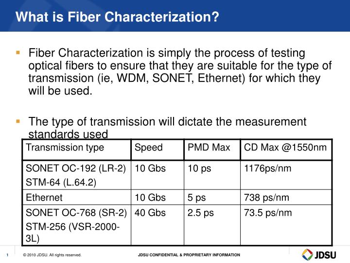
What is Fiber Characterization?. Fiber Characterization is simply the process of testing optical fibers to ensure that they are suitable for the type of transmission (ie, WDM, SONET, Ethernet) for which they will be used. The type of transmission will dictate the measurement standards used.

E N D
What is Fiber Characterization? • Fiber Characterization is simply the process of testing optical fibers to ensure that they are suitable for the type of transmission (ie, WDM, SONET, Ethernet) for which they will be used. • The type of transmission will dictate the measurement standards used
Insertion Loss (IL) Also called span loss testing
Insertion Loss or Span Loss Testing • The most important test to be performed, as each combination of transmitter/receiver has a power range limit. • ILProvides the most accurate end-to-end loss measurement of fiber optic link including end connectors. • An IL measurement requires a calibrated source and a power meter. The source sends a signal at a given power level, and the power meter reads the remaining power level at the far end of the link. • This is a unidirectional measurement, however performed bi-directionally for operation purposes
Test jumper #2 Test jumper #1 Fibre under test Calibrated light source Power Meter Total attenuation of the link Reference and Test Procedure A 2-step operation • Step 1: Reference power level: Quantify the output power including the fiber jumpers. Connect source and power meter together with the jumpers. • Step2: Insert the fiber under test and the power measurement of the connected elements (jumpers + fiber under test). Test jumpers Calibrated light source Power Meter
Optical Return Loss • The optical return loss (ORL) represents the portion of light reflected back to the transmitter by the link components (connectors…) and the fiber itself. • The 2 predominant test methods: • Optical Continuous Wave Reflectometry (OCWR) • A laser source and a power meter, using the same test port, are connected to the fiber under test. • Optical Time Domain Reflectometry (OTDR) • The OTDR is able to measure not only the total ORL of the link but also section ORL (cursor A – B) • Excess ORL can cause high BER due to transmitter instability and/or noise at the receiver via Multi-path Interference (MPI). PPC Pelement PAPC PAPC PR Transmitter (Tx) Receiver (Rx) PBS PBS PBS PT
Polarized optical signal (vector sum of the polarization modes) Polarization Mode (PSP) Polarization Mode (PSP) State of Polarization (SOP) Slow Axis PSP Fast Axis The polarization eigenmodes are represented as two propagation axes, called PSP : Principal States of Polarization.
Polarization Mode Dispersion - The Causes - • No perfect fiber circularity and symmetry (birefringence) • the group velocities of the PSPs are slightly different inducing PMD. • Fiber stress and in-homogeneity ( e.g. bends… ) create local birefringence, inducing coupling between the PSPs. • A real fiber is a randomly distribution addition of these local bi-refringence sections • Light launched into a fiber with a given state of polarization (SOP) changes its SOP along the way in a slowly time-varying random process ( i.e. unpredictable) . Local bi-refringence sections in a fiber
Why does PMD appears ? • Fiber optic cables which have been deployed in the outside plant are not perfect. • Manufacturing defects. • The fiber core is not perfectly circular along its overall length • The fiber core is not perfectly concentric with the cladding • The fiber can be twisted, tapered, or bent at some points along the span.
Perfect SM Fiber span V1 > V2 Differential Group Delay Different polarization modes travel at different velocities presenting a different propagation time between the two modes (PSPs). The resulting difference in propagation time between polarization modes is called Differential Group Delay (DGD). Standard SM fiber span DGD v2 v1
Fast Slow Strong Mode coupling Separated polarisation modes interact with each other: PSPs are changing randomly (External constraints (stress, bending, twisting), Temperature…) Birefringent sections (randomly concentrated) DGD v2 External stress !! v1
Polarization Mode Dispersion - The phenomenon - • Interaction between light and material properties: SOP vs birefringence • PMD is the average value of the Differential Group Delay (mean DGD), so called PMD delay [ps], expressed by the PMD delay coefficient c[ps/km] = • Instantaneous PMD varies with , time, T°, movement. PMD is not intrinsic and requires statistical predictions • PMD fluctuates over the network life cycle
Polarization Mode Dispersion - The Issues - • PMD constraints increase with: • Channel Bit rate • Fiber length (number of sections) • Number of channels (increase missing channel possibility) • PMD decreases with: • Better fiber manufacturing control (fiber geometry…) • PMD compensation modules • PMD is more an issues for old G652 fibers (<1996) than newer G652, G653, G655 fibers At any given signal wavelength the PMD is an unstable phenomenon, unpredictable.
PMD tolerance for NRZ transmission with 1dB power penalty PMD – Limiting Transmission Parameter -
10 Gig Ethernet transmission Limits • As defined by the IEEE 802.3ae-2002 standard, tolerances for dispersion are much lower than Sonet/SDH. • 2 principle constraints • Forward Error Correction is not robust to CD impact • Acceptable outage probability is lower • 10-7 for 10Gig Ethernet vs 10-5 for SDH/SONET
When Measuring PMD? • PMD is created or affected at different stages of the network deployment and must be measured • During the fiber manufacturing process (plant) • During the cable manufacturing process (plant) • After installation of the cable for very high bit rate (field) • 10 Gbit/s per channel or above • At the planning to upgrade an existing network (field) • Fiber manufactured before <1990 have to be verified • Regularly during the network life (environmental conditions) • Additional service to be offered by installers
PMD Testing - Equipment Overview • The broadband source sends a polarized light which is analyzed by a spectrum analyzer after passing through a polarizer • PMD measurement is typically performed unidirectional. or with T-BERD 8000 platform ODM plug-in module handheld OBS-5x0 BBS2A plug-in module When PMD results are too close to the system limits, it may be required to perform a long term measurement analysis in order to get a better picture of the variation over the time.
Test jumper Test jumper Fiber under Test PMD Testing – Equipment Setup • Measurement acquisition • Set the Broadband source mode to « PMD » • No other specific test setup, except distance… • Press and the Start the measurement • Between 6s and 12s depending on the fiber length
PMD Testing – Results Graph • FFT and associated Gaussian graphical display • Pass/Fail indication if threshold setup • Results and setting parameters automatically saved
PMD Testing – File Saving/Printing • Measurement is automatically saved in the hard disk with the associated date/time. • Autonaming setup or manual naming of traces is available if desired • Link Manager enables to get access to a quick overview of the test results
Chromatic Dispersion - The Definition - • Effect that different wavelengths (colors or spectral components of light) travel at different speed in a media (Fiber for ex.) • In telecommunications, an optical pulse is composed by multiple wavelengths which travel at different speeds. • In DWDM transmission, each wavelength/frequency (each color) travels at a different speed. • It depends on the spectral quality of the source and its modulation scheme propagation delay time due to the variation of index according to the wavelength
Chromatic Dispersion – The Parameters - • Chromatic Dispersion (CD) is measured in ps/(nm.km) and is the pulse (or group) delay (ps) of a wavelength variation of one nanometer (nm), over one km. • The chromatic dispersion value is provided at a given wavelength. • It can be positive (shorter wavelengths travelling faster) or negative (longer wavelengths travelling faster). • The zero dispersion wavelength value: 0 , in nm • The dispersion slope (S) describes the amount of CD change for different wavelengths • It is expressed in ps/(nm2.km) • The slope along the 0 wavelength: S0 , in ps/(nm2.km) • Intrinsic fiber parameter but varies with fiber type.
gives this The slope of this + S0 slope at zero dispersion zero dispersion wavelength Pulse delay (ps) Chromatic Dispersion (ps/nm-km) _ (nm) (nm) zero dispersion wavelength Zero dispersion wavelength • Wavelength where the Dispersion is null. • Operating at this wavelength does not exhibit Chromatic dispersion
Chromatic dispersion – The causes - Material dispersion 20 Total Chromatic Dispersion 20 10 1290nm Dispersion (ps/nm.km) 0 1310nm -10 Waveguide Dispersion -20 1200 1300 1400 1500 l (nm) Core refractive index Material dispersion Waveguide dispersion Index profile and MFD
At the end the pulse is larger The pulse spectrum has a width Chromatic Dispersion Blue Red Transmission starting Transmission ending 1 2 3 4 5 Chromatic Dispersion – The Phenomenon -
CD Value (ps/nm.km) 40 G652 Standard SMF ( Unshifted Dispersion) 30 G656 Non-Zero Dispersion for Wideband Transport 20 G655 Non Zero Disp. Shifted SMF 10 0 G653 Dispersion Shifted SMF 1100 1000 1200 1310 1400 1500 1600 Chromatic Dispersion – Fiber parameter - Wavelength (nm)
Chromatic Dispersion - The Effects - • The variation of index according to the wavelength induces a pulse width variation and may consequently cause it to interfere with neighboring pulses. It also reduces the pulse peak power. • It limits the transmission speed of the networks • It limits the transmission distance of the networks • It puts limits on DWDM due to relation with FWM, but this can be optimized
CD tolerance for NRZ transmission with 1dB power penalty Dispersion related system power penalty is generaly of 1dB max. Chromatic Dispersion – Limiting Transmission Parameter -
10 Gig Ethernet transmission Limits • As defined by the IEEE 802.3ae-2002 standard, tolerances for dispersion are much lower than Sonet/SDH. • 2 principle constraints • Forward Error Correction is not robust to CD impact • Acceptable outage probability is lower • 10-7 for 10Gig Ethernet vs 10-5 for SDH/SONET
Distance (Km) = Specification of Transponder (ps/nm) Coef.of Dispersion of Fiber (ps/nm*km) A receiver with dispersion tolerance of 3400 ps/nm is sent across a standard SMF-28 fiber which has a Coefficient of Dispersion of 17 ps/nm*km. It will reach 200 Km at maximum bandwidth. (Note that lower speeds will travel farther.) How far can I go without dispersion compensation?
Dealing with Chromatic Dispersion • These parameters can be controlled in such way to control the material dispersion: • Using of fiber which has minimum dispersion. • Selecting a low chirp source • Using external modulator • Using electronic regenerator (high cost). • Using dispersion compensation.
Chromatic Dispersion – Equipment Overview • The CD test set consists of a broadband light source (transmitter) and a phase meter (receiver) connected at each end of the fiber under test. The receiver measures the broadband signal in user defined increments (such as10 nm increments). Approximation formula is then applied in order to calculate the dispersion over a given wavelength range. • CD measurement is typically performed unidirectional. or with T-BERD 8000 platform ODM plug-in module handheld OBS-5x0 BBS2A plug-in module The results will be correlated to the transmission system limits according to the bit rate being implemented.
Chromatic Dispersion Testing – Equipment Setup • Source referencing • To be performed in order to calibrate the receiver with the Broadband Source • At the early begining of a measurement campaign • Connect the test jumpers to the source and the ODM module • In the CD Setup page, Press the soft key « Acq. Ref », select Yes to perform a new reference, enter the source serial number and confirm. • A green « valid reference » indicator will be displayed at the end of the reference acqusition. Test jumpers • Measurement acquisition • Connect both instruments at each end of the fiber under test using the calibrated test jumpers. • Press to perform the acqusition • Between 45s and 70s depending on the fiber length Test jumper Test jumper Fiber under Test
Chromatic Dispersion Testing – Results Graph Dispersion curve Zero dispersion wavelength and slope CD value vs. wavelength: • Total link dispersion per wavelength • Dispersion slope The Chromatic dispersion measurement will be performed over a given wavelength range and results will be correlated to the transmission system limits according to the bit rate being implemented.
Chromatic Dispersion Testing – File Saving/Printing • Measurement is automatically saved in the hard disk with the associated date/time. • Autonaming setup or manual naming of traces is available if desired • Link Manager enables to get access to a quick overview of the test results
Fiber Attenuation vs. Wavelength • Attenuation depends on the fiber type and the wavelength. If the absorption spectrum of a fiber is plotted against the wavelength of the laser, certain characteristics of the fiber can be identified. • The graph in Figure 2 illustrates the relationship between the wavelength of the injected light and the total fiber attenuation.
Why measuring Attenuation Profile of a fiber? • The purpose of the AP measurement is to represent the attenuation as a function of the wavelength. • Historically, this measurement was required mainly for long-haul applications. Meanwhile, with the increase of CWDM deployment and the extension of the DWDM wavelength range, it is becoming necessary to have a clear picture of the fiber attenuation other the wavelengths intended to be filled-in with traffic.
Characterizing the full wavelength range • In long distance transmissions, as well as at very high bit rate (10G, 40G systems), Raman amplifications are more and more in use. In addition, new Distal pumping of Erbium amplifiers at 1480 nm are currently deployed. Characterizing fiber at the pump wavelengths (1420, 1450 nm, 1480 nm, etc.) is of high interest to ensure amplification will occur along the required distance. • Because all of these applications make such a broad and varied use of the optical fiber, characterization over the complete useful wavelength is justified rather than characterizing only at discrete wavelengths.
Attenuation Profile • An AP test set consists of a broadband light source (transmitter) and a spectrum analyzer (receiver). The broadband source sends light, with a given wavelength range, into the fiber under test, which is analyzed by the spectrum analyzer at the far end. or with T-BERD 8000 platform ODM plug-in module handheld OBS-5x0 BBS2A plug-in module Every fiber presents varying levels of attenuation across the transmission spectrum. The purpose of the AP measurement is to represent the attenuation as a function of the wavelength.
Test jumper Test jumper Test jumper Fiber under Test Attenuation Profile Testing – Equipment Setup • Source referencing • To be performed in order to measure the Broadband Source output power with test jumpers • At the early begining of a measurement campaign • Each time jumpers are changed/disconnected • Connect the test jumpers to the source and the ODM module • In the AP Setup page, Press the soft key « Acq. Ref », select Yes to perform a new reference, enter the source serial number and confirm. • Measurement acquisition • Set the Broadband source mode to « AP » • No specific test setup, except distance…Just press Start ! • After 12s max.
Attenuation Profile Testing – Results Graph Attenuation profile curve Loss value vs. wavelength: • Coefficient (dB/km) • Total link loss per wavelength (dB)
Attenuation Profile Testing – File Saving/Printing • Measurement is automatically saved in the hard disk with the associated date/time. • Autonaming setup or manual naming of traces is available if desired • Link Manager enables to get access to a quick overview of the test results