Download
1 / 9
90 likes | 156 Vues
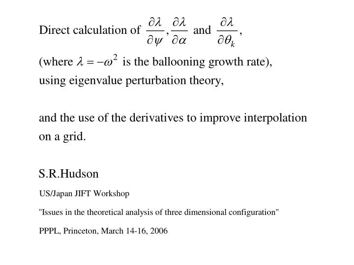
From local to global : ray tracing. with grid spacing h. Alternatively, the eigenvalue derivatives can be determined directly using perturbation theory. The direct calculation of the derivatives is beneficial because. The rays may be integrated directly the data-cube need not be constructed

E N D
From local to global : ray tracing with grid spacing h
Alternatively, the eigenvalue derivatives can be determined directly using perturbation theory
The direct calculation of the derivatives is beneficial because . . . • The rays may be integrated directly • the data-cube need not be constructed • the eigenvalue derivatives may be given directly to an o.d.e. integrator • this may be useful if only a few ray trajectories are required • simple to locally refine ray trajectories using higher numerical accuracy • The calculation of the derivatives is consistent with the calculation of the eigenvalue • The derivatives enable a higher order interpolation of the data-cube. • Consider a 2 point interpolation in 1 dimension,
For example, consider a tokamak • A circular cross section tokamak is simple • there is no dependence, minimal #Fourier harmonics • note that the ballooning code, interpolation, ray tracing etc. is fully 3D • Shown below are unstable ballooning contours
In 3D, 4th order interpolation is easily obtained eigenvalue interpolation error derivative interpolation error
The use of the derivatives enables a crude-grid to give good interpolation solid : exact calculated at 100 radial points dashed : 2-point interpolation ballooning profile X : grid points X : grid points radial (VMEC) coordinate
k s Construction of data-cube allows eigenvalue iso-sufaces to be visualized Another example : LHD variant studied by Nakajima et al. ISW 2005 as eigenvalue is increased, iso-sufaces become more localized
Future work possibly includes . . . • compare results of ray-tracing to global stability results • investigate discrepancy between local and global stability limits • appropriate mass normalization for comparison with CAS3D / TERPSICHORE • include FLR effects / chaotic ray-dynamics as studied by MacMillan & Dewar