Download

1 / 85
860 likes | 999 Vues
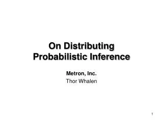
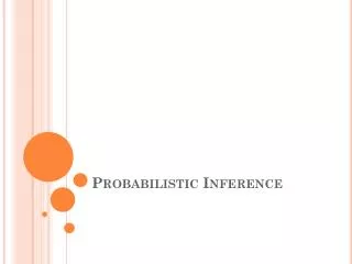
Probabilistic Inference Lecture 2. M. Pawan Kumar pawan.kumar@ecp.fr. Slides available online http:// cvc.centrale-ponts.fr /personnel/ pawan /. Pose Estimation. Courtesy Pedro Felzenszwalb. Pose Estimation. Courtesy Pedro Felzenszwalb. Pose Estimation. Variables are body parts.

E N D
Probabilistic InferenceLecture 2 M. Pawan Kumar pawan.kumar@ecp.fr Slides available online http://cvc.centrale-ponts.fr/personnel/pawan/
Pose Estimation Courtesy Pedro Felzenszwalb
Pose Estimation Courtesy Pedro Felzenszwalb
Pose Estimation Variables are body parts Labels are positions
Pose Estimation Variables are body parts Labels are positions Unary potentials θa;i proportional to fraction of foreground pixels
Pose Estimation Head Joint location according to ‘head’ part d Joint location according to ‘torso’ part Torso Pairwise potentials θab;ik proportional to d2
Pose Estimation Head Head d > d Torso Torso Pairwise potentials θab;ik proportional to d2
Outline • Problem Formulation • Energy Function • Energy Minimization • Computing min-marginals • Reparameterization • Energy Minimization for Trees • Loopy Belief Propagation
Energy Function Label l1 Label l0 Vb Vc Vd Va Random Variables V= {Va, Vb, ….} Labels L= {l0, l1, ….} Labelling f: {a, b, …. } {0,1, …}
Energy Function 6 3 2 4 Label l1 Label l0 5 3 7 2 Vb Vc Vd Va Easy to minimize Q(f) = ∑a a;f(a) Neighbourhood Unary Potential
Energy Function 6 3 2 4 Label l1 Label l0 5 3 7 2 Vb Vc Vd Va E : (a,b) E iff Va and Vb are neighbours E = { (a,b) , (b,c) , (c,d) }
Energy Function 0 6 1 3 2 0 4 Label l1 1 2 3 4 1 1 Label l0 1 0 5 0 3 7 2 Vb Vc Vd Va Pairwise Potential Q(f) = ∑a a;f(a) +∑(a,b) ab;f(a)f(b)
Energy Function 0 6 1 3 2 0 4 Label l1 1 2 3 4 1 1 Label l0 1 0 5 0 3 7 2 Vb Vc Vd Va Q(f; ) = ∑a a;f(a) +∑(a,b) ab;f(a)f(b) Parameter
Outline • Problem Formulation • Energy Function • Energy Minimization • Computing min-marginals • Reparameterization • Energy Minimization for Trees • Loopy Belief Propagation
Energy Minimization 0 6 1 3 2 0 4 Label l1 1 2 3 4 1 1 Label l0 1 0 5 0 3 7 2 Vb Vc Vd Va Q(f; ) = ∑a a;f(a) + ∑(a,b) ab;f(a)f(b)
Energy Minimization 0 6 1 3 2 0 4 Label l1 1 2 3 4 1 1 Label l0 1 0 5 0 3 7 2 Vb Vc Vd Va Q(f; ) = ∑a a;f(a) + ∑(a,b) ab;f(a)f(b) 2 + 1 + 2 + 1 + 3 + 1 + 3 = 13
Energy Minimization 0 6 1 3 2 0 4 Label l1 1 2 3 4 1 1 Label l0 1 0 5 0 3 7 2 Vb Vc Vd Va Q(f; ) = ∑a a;f(a) + ∑(a,b) ab;f(a)f(b)
Energy Minimization 0 6 1 3 2 0 4 Label l1 1 2 3 4 1 1 Label l0 1 0 5 0 3 7 2 Vb Vc Vd Va Q(f; ) = ∑a a;f(a) + ∑(a,b) ab;f(a)f(b) 5 + 1 + 4 + 0 + 6 + 4 + 7 = 27
Energy Minimization 0 6 1 3 2 0 4 Label l1 1 2 3 4 1 1 Label l0 1 0 5 0 3 7 2 Vb Vc Vd Va q* = min Q(f; ) = Q(f*; ) Q(f; ) = ∑a a;f(a) + ∑(a,b) ab;f(a)f(b) f* = arg min Q(f; )
Energy Minimization f* = {1, 0, 0, 1} 16 possible labellings q* = 13
Outline • Problem Formulation • Energy Function • Energy Minimization • Computing min-marginals • Reparameterization • Energy Minimization for Trees • Loopy Belief Propagation
Min-Marginals 0 6 1 3 2 0 4 Label l1 1 2 3 4 1 1 Label l0 1 0 5 0 3 7 2 Vb Vc Vd Va such that f(a) = i f* = arg min Q(f; ) Min-marginal qa;i
Min-Marginals qa;0 = 15 16 possible labellings
Min-Marginals qa;1 = 13 16 possible labellings
Min-Marginals and MAP • Minimum min-marginal of any variable = • energy of MAP labelling qa;i mini ) mini ( such that f(a) = i minfQ(f; ) Va has to take one label minfQ(f; )
Summary Energy Function Q(f; ) = ∑a a;f(a) + ∑(a,b) ab;f(a)f(b) Energy Minimization f* = arg min Q(f; ) Min-marginals s.t. f(a) = i qa;i= min Q(f; )
Outline • Problem Formulation • Reparameterization • Energy Minimization for Trees • Loopy Belief Propagation
Reparameterization 2 + - 2 2 0 4 1 1 2 + - 2 5 0 2 Vb Va Add a constant to all a;i Subtract that constant from all b;k
Reparameterization 2 + - 2 2 0 4 1 1 2 + - 2 5 0 2 Vb Va Add a constant to all a;i Subtract that constant from all b;k Q(f; ’) = Q(f; )
Reparameterization + 3 - 3 2 0 4 - 3 1 1 5 0 2 Vb Va Add a constant to one b;k Subtract that constant from ab;ik for all ‘i’
Reparameterization + 3 - 3 2 0 4 - 3 1 1 5 0 2 Vb Va Add a constant to one b;k Subtract that constant from ab;ik for all ‘i’ Q(f; ’) = Q(f; )
3 1 3 1 3 0 1 1 1 2 2 4 2 4 2 4 0 1 2 1 5 0 5 5 2 2 2 Vb Vb Vb Va Va Va Reparameterization - 4 + 4 + 1 - 4 - 2 - 1 + 1 - 2 - 4 + 1 - 2 + 2 + Mab;k + Mba;i ’b;k = b;k ’a;i = a;i Q(f; ’) = Q(f; ) ’ab;ik = ab;ik - Mab;k - Mba;i
Equivalently 2 + - 2 2 0 4 + Mba;i ’a;i = a;i 1 1 + Mab;k 2 + - 2 5 0 2 Vb Va ’ab;ik = ab;ik - Mab;k - Mba;i Reparameterization ’ is a reparameterization of , iff ’ Q(f; ’) = Q(f; ), for all f Kolmogorov, PAMI, 2006 ’b;k = b;k
Recap Energy Minimization f* = arg min Q(f; ) Q(f; ) = ∑a a;f(a) + ∑(a,b) ab;f(a)f(b) Min-marginals s.t. f(a) = i qa;i= min Q(f; ) Reparameterization ’ Q(f; ’) = Q(f; ), for all f
Outline • Problem Formulation • Reparameterization • Energy Minimization for Trees • Loopy Belief Propagation Pearl, 1988
Belief Propagation • Some problems are easy • Belief Propagation is exact for chains • Exact MAP for trees • Clever Reparameterization
Two Variables 2 2 0 4 1 1 5 0 5 2 Vb Vb Va Va Add a constant to one b;k Subtract that constant from ab;ik for all ‘i’ ’b;k = qb;k Choose the right constant
Two Variables 2 2 0 4 1 1 5 0 5 2 Vb Vb Va Va = 5 + 0 a;0 + ab;00 Mab;0 = min = 2 + 1 a;1 + ab;10 ’b;k = qb;k Choose the right constant
Two Variables 2 2 0 4 1 -2 5 -3 5 5 Vb Vb Va Va ’b;k = qb;k Choose the right constant
Two Variables f(a) = 1 2 2 0 4 1 -2 5 -3 5 5 Vb Vb Va Va ’b;0 = qb;0 Potentials along the red path add up to 0 ’b;k = qb;k Choose the right constant
Two Variables 2 2 0 4 1 -2 5 -3 5 5 Vb Vb Va Va = 5 + 1 a;0 + ab;01 Mab;1 = min = 2 + 0 a;1 + ab;11 ’b;k = qb;k Choose the right constant
Two Variables f(a) = 1 f(a) = 1 2 2 -2 6 -1 -2 5 -3 5 5 Vb Vb Va Va ’b;0 = qb;0 ’b;1 = qb;1 Minimum of min-marginals = MAP estimate ’b;k = qb;k Choose the right constant
Two Variables f(a) = 1 f(a) = 1 2 2 -2 6 -1 -2 5 -3 5 5 Vb Vb Va Va ’b;0 = qb;0 ’b;1 = qb;1 f*(b) = 0 f*(a) = 1 ’b;k = qb;k Choose the right constant
Two Variables f(a) = 1 f(a) = 1 2 2 -2 6 -1 -2 5 -3 5 5 Vb Vb Va Va ’b;0 = qb;0 ’b;1 = qb;1 We get all the min-marginals of Vb ’b;k = qb;k Choose the right constant
+ Mab;k ’b;k= b;k + Mba;i ’a;i = a;i ’ab;ik = ab;ik - Mab;k - Mba;i Recap We only need to know two sets of equations General form of Reparameterization Reparameterization of (a,b) in Belief Propagation Mab;k = mini { a;i + ab;ik } Mba;i = 0
Three Variables 0 2 4 0 6 l1 3 1 1 2 l0 5 0 1 3 2 Vb Vc Va Reparameterize the edge (a,b) as before
Three Variables f(a) = 1 -2 2 6 0 6 l1 3 -2 -1 2 l0 5 -3 1 3 5 Vb Vc Va f(a) = 1 Reparameterize the edge (a,b) as before
Three Variables f(a) = 1 -2 2 6 0 6 l1 3 -2 -1 2 l0 5 -3 1 3 5 Vb Vc Va f(a) = 1 Reparameterize the edge (a,b) as before Potentials along the red path add up to 0
Three Variables f(a) = 1 -2 2 6 0 6 l1 3 -2 -1 2 l0 5 -3 1 3 5 Vb Vc Va f(a) = 1 Reparameterize the edge (b,c) as before Potentials along the red path add up to 0
Three Variables f(a) = 1 f(b) = 1 -2 2 6 -6 12 l1 -3 -2 -1 -4 l0 5 -3 -5 9 5 Vb Vc Va f(a) = 1 f(b) = 0 Reparameterize the edge (b,c) as before Potentials along the red path add up to 0