Download
1 / 54
540 likes | 548 Vues
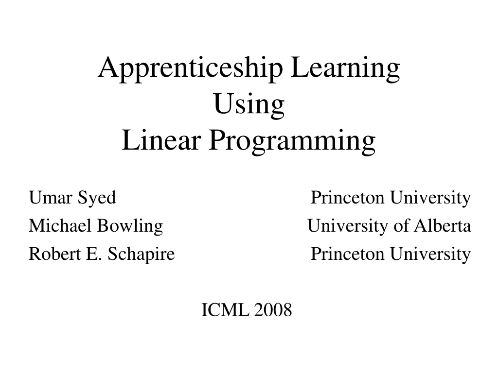
Apprenticeship Learning Using Linear Programming. ICML 2008. Apprenticeship Learning: An apprentice learns to behave by observing an expert. Learning algorithm. Output : Apprentice policy that is at least as good as expert policy (and possibly better).

E N D
Apprenticeship Learning: An apprentice learns to behave by observing an expert. Learning algorithm Output: Apprentice policy that is at least as good as expert policy (and possibly better). Input: Demonstrations by expert policy.
Main Contribution A new apprenticeship learning algorithm that: Produces simpler apprentice policies, and Is empirically faster than previous algorithms.
Outline Introduction Apprenticeship Learning Prior Work Summary of Advantages Over Prior Work Background: Occupancy Measure Linear Program for Apprenticeship Learning (LPAL) Experiments and Demos Other Topics
Given:Same as Markov Decision Process, except no reward function R. Also given: Basis reward functions R1, …, Rk. Demonstrations by an expert policy ¼E. Assume: True reward function R is a weighted combination of the k basis reward functions: R(s, a) = iwi* ¢ Ri(s, a) where weight vector w* is unknown. Goal: Find apprentice policy ¼A such that V(¼A) ¸ V(¼E) where value V(¼) of policy ¼ is with respect to unknown reward function. Apprenticeship Learning
Outline Introduction Apprenticeship Learning Prior Work Summary of Advantages Over Prior Work Background: Occupancy Measure Linear Program for Apprenticeship Learning (LPAL) Experiments and Demos Other Topics
Define Vi(¼) = ith “basis value” of ¼ = Value of ¼ with respect to ith basis reward function. Then true value of a policy is a weighted combination of its basis values, i.e. V(¼) = iwi*¢Vi(¼) Proof: Linearity of expectation. Prior Work – Key Idea
Introduced the apprenticeship learning framework. Algorithm Idea: Estimate Vi(¼E) for all i from expert’s demonstrations. Find ¼A such that Vi(¼A) = Vi(¼E) for all i. Theorem: V(¼A) = V(¼E) Algorithm “type”:Geometric Prior Work – Abbeel & Ng (2004)
Assumed that all wi* are non-negative and sum to 1. Algorithm Idea: Estimate Vi(¼E) for all i from expert’s demonstrations. Find ¼A and M such that: Vi(¼A) ¸Vi(¼E) + M for all i, and M is as large as possible. Theorem: V(¼A) ¸ V(¼E), and possibly V(¼A) À V(¼E). Algorithm “type”:Boosting Prior Work – Syed & Schapire (2007)
Outline Introduction Apprenticeship Learning Prior Work Summary of Our Approach Background: Occupancy Measure Linear Program for Apprenticeship Learning (LPAL) Experiments and Demos Other Topics
Same algorithm idea as Syed & Schapire (2007), but formulated as a single linear program, which we give to an off-the-shelf solver. Summary of Our Approach
Previous algorithms: Didn’t actually output a single stationary policy ¼A, but instead output a distributionD over a set of stationary policies, such that E¼ »D[V(¼A)] ¸ V(¼E) Our algorithm: Outputs a single stationary policy ¼A such that V(¼A) ¸ V(¼E), and possibly V(¼A) À V(¼E). Advantage: Apprentice policy is simpler and more intuitive. Advantages of Our Approach A
Advantages of Our Approach • Previous algorithms: Ran for several rounds, and each round required solving a standard MDP (expensive). • Our algorithm: A single linear program. • Advantage: Empirically faster than previous algorithms. • We informally conjecture that this is because it solves the problem “all at once”.
Outline Introduction Apprenticeship Learning Prior Work Summary of Our Approach Background: Occupancy Measure Linear Program for Apprenticeship Learning (LPAL) Experiments and Demos Other Topics
The occupancy measurex¼2R|S||A| of policy ¼is an alternate way of describing how ¼ moves through the state-action space. x¼sa = Expected (discounted) number of visits by policy ¼ to state-action pair (s, a). Example: Suppose policy ¼ visits state-action pair (s, a): With probability 1 at time 1. With probability 1/2 at time 2. With probability 1/3 at time 3. With probability 0 a time ¸ 4. Then x¼sa = 1 + °(1/2) + °2(1/3) Occupancy Measure
Occupancy Measure – Equivalent Representation The relationship between a stationary policy ¼and its occupancy measure x¼is given by: Proof: Left-hand side = Probability of taking action a in state s. Right-hand side = No. of visits to state-action (s, a) No. of visits to state s. Significance: It is easy to recover a stationary policy from its occupancy measure.
Define º(x) ,s,a R(s, a) ¢xsa Then V(¼) = º(x¼). In other words, º(x) is the value of a policy whose occupancy measure is x. Proof: A policy earns reward R(s, a) (suitably discounted) every time it visits state-action pair (s, a). Significance: The value of a policy is a linear function of its occupancy measure. Occupancy Measure – Calculating Value
Occupancy Measure – Bellman Flow Constraints The Bellman flow constraints are a set of constraints that any vector x2R|S||A| must satisfy to be a valid occupancy measure. The Bellman flow constraints say: “Under any policy, the number of visits into a state s must equal the number of visits leaving state s.” s Must be equal
Occupancy Measure – Bellman Flow Constraints In fact, the Bellman flow constraints completely characterize the set of occupancy measures. x satisfies the Bellman flow constraints m x is the occupancy measure of some policy ¼ Significance: The Bellman flow constraints are linear in x. All policies All occupancy measures ¢¼ x ¢ Bellman flow constraints
Outline Introduction Apprenticeship Learning Prior Work Summary of Our Approach Background: Occupancy Measure Linear Program for Apprenticeship Learning (LPAL) Experiments and Demos Other Topics
Derivation of LPAL Algorithm 1. Estimate Vi(¼E) for all i from expert’s demonstrations. 2. Find ¼A and M that solve: max M subject to: Vi(¼A) - Vi(¼E) ¸ M for all i. ¼A is a policy. Start with algorithm idea from Syed & Schapire (2007)
Derivation of LPAL Algorithm 1. Estimate Vi(¼E) for all i from expert’s demonstrations. 2. Find ¼A and M that solve: max M subject to: Vi(¼A) - Vi(¼E) ¸ M for all i. ¼A is a policy. xA satisfies the Bellman flow constraints. xA
Derivation of LPAL Algorithm 1. Estimate Vi(¼E) for all i from expert’s demonstrations. 2. Find ¼A and M that solve: max M subject to: Vi(¼A) - Vi(¼E) ¸ M for all i. ¼A is a policy. xA satisfies the Bellman flow constraints. xA ºi(xA)
Derivation of LPAL Algorithm 1. Estimate Vi(¼E) for all i from expert’s demonstrations. 2. Find¼Aand M that solve: max M subject to: Vi(¼A) - Vi(¼E) ¸ M for all i. ¼A is a policy xA satisfies the Bellman flow constraints. xA ¼A ºi(xA) Vi(¼A) ¼A is a policy.
Derivation of LPAL Algorithm 1. Estimate Vi(¼E) for all i from expert’s demonstrations. 2. Find xA and M that solve: max M subject to: ºi(xA) - Vi(¼E) ¸ M for all i. xA satisfies the Bellman flow constraints.
Derivation of LPAL Algorithm 1. Estimate Vi(¼E) for all i from expert’s demonstrations. 2. Find xA and M that solve: max M subject to: ºi(xA) - Vi(¼E) ¸ M for all i. xA satisfies the Bellman flow constraints. This is a linear program!
Derivation of LPAL Algorithm 1. Estimate Vi(¼E) for all i from expert’s demonstrations. 2. Find xA and M that solve: max M subject to: ºi(xA) - Vi(¼E) ¸ M for all i. xA satisfies the Bellman flow constraints. “Of all occupancy measures …
Derivation of LPAL Algorithm 1. Estimate Vi(¼E) for all i from expert’s demonstrations. 2. Find xA and M that solve: max M subject to: ºi(xA) - Vi(¼E) ¸ M for all i. xA satisfies the Bellman flow constraints. “Of all occupancy measures … find one corresponding to a policy that is better than the expert’s policy …
Derivation of LPAL Algorithm 1. Estimate Vi(¼E) for all i from expert’s demonstrations. 2. Find xA and M that solve: max M subject to: ºi(xA) - Vi(¼E) ¸ M for all i. xA satisfies the Bellman flow constraints. “Of all occupancy measures … find one corresponding to a policy that is better than the expert’s policy … by as much as possible.”
Derivation of LPAL Algorithm 1. Estimate Vi(¼E) for all i from expert’s demonstrations. 2. Find xA and M that solve: max M subject to: ºi(xA) - Vi(¼E) ¸ M for all i xA satisfies the Bellman flow constraints. “Of all occupancy measures … find one corresponding to a policy that is better than the expert’s policy … by as much as possible.” 3. Convert occupancy measure to a stationary policy:
Theorem: V(¼A) ¸ V(¼E), and possibly V(¼A) À V(¼E). (same as Syed & Schapire (2007)) Proof: Almost immediate. Remark: We could have applied the same occupancy measure “trick” to the algorithm idea from Abbeel & Ng (2004), and likewise derived a linear program. LPAL Algorithm
Outline Introduction Apprenticeship Learning Prior Work Summary of Our Approach Background: Occupancy Measure Linear Program for Apprenticeship Learning (LPAL) Experiments and Demos Other Topics
Experiment – Setup • Actions & transitions: North, South, East and West, with 30% chance of moving to a random state. • Basis rewards: One indicator basis reward per region. • Expert: Optimal policy for randomly chosen weight vector w*. “Gridworld” environment, divided into regions Region State
Experiment – Setup • Compare: • Projection algorithm (Abbeel & Ng 2004) • MWAL algorithm (Syed & Schapire 2007) • LPAL algorithm (this work) • Evaluation Metric: Time required to learn apprentice policy whose value is 95% of the optimal value.
Experiment – Results Note: Y-axis is log scale.
Experiment – Results Note: Y-axis is log scale.
Demo – Mimicking the Expert Output of LPAL algorithm Expert
Demo – Improving Upon the Expert Output of LPAL algorithm Expert
Outline Introduction Apprenticeship Learning Prior Work Summary of Our Approach Background: Occupancy Measure Linear Program for Apprenticeship Learning (LPAL) Experiments and Demos Other Topics
Also Discussed in the Paper… • We observe that the MWAL algorithm often performs better than its theory predicts it should. • We have new results explaining this behavior (in preparation).
Constrained MDPs and RL with multiple rewards: Feinberg and Schwartz (1996) Gabor, Kalmar and Szepesvari (1998) Altman (1999) Shelton (2000) Dolgov and Durfree (2005) … Max margin planning: Ratliff, Bagnell and Zinkevich (2006) Related to Our Approach
Recap A new apprenticeship learning algorithm that: Produces simpler apprentice policies, and Is empirically faster than previous algorithms. Thanks! Questions?
Algorithms for finding ¼A: Max-Margin: Based on quadratic programming. Projection: Based on a geometric approach. MWAL: Based on a multiplicative weights approach, similar to boosting. Actually, existing algorithms don’t find a single stationary ¼A, but instead find a distributionD over a set of stationary policies, such that E¼»D[V(¼A)] ¸ V(¼E). Drawbacks: Apprentice policy is nonintuitive and complicated to describe. Algorithms have slow empirical running time. Prior Work – Details
Same algorithm idea: Find ¼A such that Vi(¼A) ¸Vi(¼E) for all i. Algorithm to find ¼A based on linear programming. Allows us to leverage the efficiency of modern LP solvers. Outputs a single stationary policy ¼A such that V(¼A) ¸ V(¼E). Benefits: Apprentice policy is simpler. Algorithm is empirically much faster. This Work
Same algorithm idea: Find ¼A such that Vi(¼A) ¸Vi(¼E) for all i. Algorithm to find ¼A based on linear programming. Allows us to leverage the efficiency of modern LP solvers. Outputs a single stationary policy ¼A such that V(¼A) ¸ V(¼E). Benefits: Apprentice policy is simpler. Algorithm is empirically much faster. This Work
The occupancy measurex¼2R|S||A| of policy ¼is an alternate way of describing how ¼ moves through the state-action space. x¼sa = Expected (discounted) number of visits by policy ¼ to state-action pair (s, a). Occupancy Measure – Equivalent Representation
Given the occupancy measure x¼of a policy ¼, computing the basis values of ¼is easy. Define ºi(x) ,s,a Ri(s, a) ¢xsa Then V_i(\pi) = \nu_i(x^\pi). In other words, \nu_i(x) is the ith basis value of a policy whose occupancy measure is x. Proof: Policy ¼ earns (suitably discounted) reward Ri(s, a) for each visit to state-action pair (s, a). And x¼sa is the expected (and suitably discounted) number of visits by policy ¼ to state-action pair (s, a). Occupancy Measure – Calculating Value
Occupancy Measure – Calculating Value Given the occupancy measure x¼of a policy ¼, computing the basis values of ¼is easy: Vi(¼) = s,a Ri(s, a) ¢x¼(s, a) Proof: Linearity of expectation. For convenience, define: ºi(x) , s,a Ri(s, a) ¢x(s, a)
Define º(x) ,s,a R(s, a) ¢xsa Then V(¼) = º(x¼). In other words, º(x) is the value of a policy whose occupancy measure is x. Proof: Policy ¼ earns (discounted) reward R(s, a) for each visit to state-action pair (s, a). And x¼sa is the expected (discounted) number of visits by policy ¼ to state-action pair (s, a). So V(\pi) is Occupancy Measure – Calculating Value
Occupancy Measure – Bellman Flow Constraints The Bellman flow constraints are a set of linear constraints that define the set of all occupancy measures. x satisfies the Bellman flow constraints m x is the occupancy measure of some policy ¼ All policies All occupancy measures ¢¼ x ¢ Bellman flow constraints