Download
1 / 47
500 likes | 756 Vues
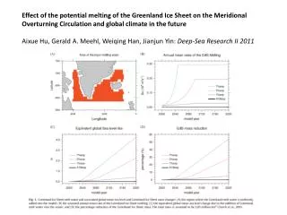
Decadal Variability of the Atlantic Meridional Overturning Circulation (AMOC). Martha Weaver Buckley (MIT). Role of the AMOC in Climate. In the mean, the Atlantic Ocean transports 1.5 PW of heat northward.

E N D
Decadal Variability of the Atlantic Meridional Overturning Circulation (AMOC) Martha Weaver Buckley (MIT)
Role of the AMOC in Climate • In the mean, the Atlantic Ocean transports 1.5 PW of heat northward. • 60% of the ocean heat transport is associated with a circulation that reaches the cold waters of the abyss (Ferrari and Ferreira, submitted). Ocean Heat Transport from NCEP Trenberth and Caron, 2001 => The deep MOC in the Atlantic plays a role in maintaining the current climate. AMOC variability may play a role in climate variability. (my focus: decadal timescales)
AMOC variability temperature anomalies Decadal AMOC variability => ocean heat transport => SST anomalies “Atlantic Multidecadal Oscillation (AMO), Kerr 2000 -0.6oC 0.6oC Decadal temperature anomalies in N. Atlantic from COADS obs. (Kushnir, 1997).
AMOC Variability temperature anomalies AMOC index and Heat Transport at 30oN 1.1 PW 18 Sv 14 Sv 0.9 PW Models show AMOC variability associated with decadal SST anomalies 1400 year control run from HadCM3 (Knight et al, 2005) Surface temperature anomalies MOC anomalies
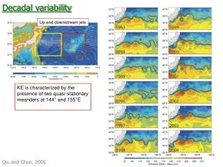
Density anomalies AMOC variability 40 Sv -20 Sv 2005 2006 2008 2007 Zonally integrated thermal wind relation: Overturning streamfunction can be reconstructed from thermal wind component, Ekman, and External mode: √ RAPID Program: MOC timeseries at 26.5oN
Our approach Toy models Simple Complex • Explore decadal density and MOC variability in a simplified setting. • Several coupled and ocean-only GCMs, idealized geometry. • Models are simple enough to isolate mechanisms. • Models are complex enough to exhibit interesting (and perhaps realistic) behavior Coupled and ocean-only GCM’s run in idealized geometries Everything should be made as simple as possible, but not simpler. --Albert Einstein
Outline • Introduction to model • Decadal Variability in idealized models (Flat, bowl) • Decadal variability of MOC • Decadal buoyancy anomalies • Relationship between buoyancy and AMOC anomalies • Role of convection • Mechanisms of decadal variability • Does AMOC play an active role in the oscillation? • Role of atmospheric forcing in mode of variability. • Source of energy for oscillations • Conclusions • Summary of decadal variability in idealized models • Using idealized models as a prism for understanding decadal variability in more complex models and data.
The Model Simple Complex “Double Drake” model • Fully coupled MITgcm: realistic 3D atmospheric & ocean • Idealized geometry: • All water except 2 ridges extending from N. Pole to 34oS • 2 types of bathymetry • Flat, with depth of 3km • Bowl shaped, depth 2.5-3km • A&O: cubed sphere grid at C24 Resolution: 3.75o latitude at equator • 5 level atmosphere, primitive equations (SPEEDY) • 15 level ocean • Diapynal mixing, constant diffusivity of 3x10⁻⁵m2s-1 • Parameterized eddies (G&M) • Convective adjustment • Integrated from rest to quasi-equilibrium Toy models Double Drake w/ bowl bathymetry Flat Double Drake
Double Drake: Mean State • Asymmetry btw hemispheres • S. Pole colder than N. Pole • Icecap over S. Pole • Fresh large basin (LB) is primarily wind-driven • Salty small basin (SB) with meridional overturning circulation (MOC) • Heat transport: • LB: Ekman and gyres, poleward both hemispheres • SB: Northward in both hemispheres due to contribution of MOC • Small basin ~ Atlantic D. Ferreira et al., 2010 (J.Climate)
MOC Variability in the small basin • Timeseries of MOC in box: 8oS to 50oN, 460 to 1890 m depth • At each latitude, chose the value of the streamfunction at the depth of the maximum of mean streamfunction. • Average over all latitudes in box.
Buoyancy anomalies in the small basin FLAT: First 2 EOFs 57% of variance 1/4 out of phase propagating mode Correlation between WBB and PC1: 0.9 with PC1 at lag=3 yrs BOWL: First 2 EOFs 41% of variance Correlation between WBB index and PC1: 0.9 at lag=0 yrs
Flat: Buoyancy anomalies and air-sea fluxes 8 W/m2 In to ocean Out of ocean -8 W/m2 -0.6oC 0.6oC
Baroclinic Rossby Waves Phase speeds: OBSERVED: c=0.47 cm/s RESTING: cR=0.15 cm/s FULL CALC: l=0: cR=0.72 cm/s l=k: cR=1.0 cm/s
Origin of buoyancy anomalies Origin, spatial pattern, and spectra of buoyancy anomalies changes with bathymetry. • Flat: • Eastern boundary is baroclinically unstable and radiates baroclinic Rossby waves, which propagate westwards. • Timescale of oscillation is set by time it takes for waves to cross basin (34 years). Bowl: • Western boundary is baroclinically unstable. • Largest buoyancy variability is constrained to the western boundary. • Variability is less regular.
Boundary buoyancy and the MOC Zonally integrated thermal wind relation: In NH: Positive MOC anomaly Negative MOC anomaly
Potential Vorticity (PV) Anomalies Less stratified More stratified Buoyancy and PV anomalies at 60oN Flat Bowl
Summary of decadal variability • Decadal MOC variability is associated with decadal buoyancy anomalies on the western boundary. • Upper ocean buoyancy anomalies exist in subpolar gyre, despite damping by air-sea buoyancy fluxes. • Increased (decreased) convection observed in areas with negative (positive) PV anomalies, as expected via preconditioning. • Anomalies move southward at depth along the western boundary. • Buoyancy anomalies lead to spin up/down the interhemispheric MOC according to the thermal wind relation. • Negative PV anomalies are associated with a stronger DWBC and MOC, in accord with observations (Line W, Pena-Molino, 2010). • MOC responds passively to buoyancy anomalies on western boundary. • Despite different origin, spatial pattern, and spectra of buoyancy anomalies in Flat and Bowl, in both models the MOC responds to buoyancy anomalies on the western boundary in the same way.
Outlook MOC variability in idealized models may be used as a prism for understanding MOC variability in more complex models & data. • Response of MOC to buoyancy anomalies • Role of MOC in creating decadal buoyancy anomalies • Role of convection in MOC variability.
Response of MOC to buoyancy anomalies MOC variability is sensitive to buoyancy anomalies in western part of basin on boundary between the subtropical & subpolar gyres. This is precisely region where significant buoyancy variability is observed in both models and data! Standard deviation of Jan–Mar SST from NCEP–NCAR reanalysis I for 1948–2006. SST is low-pass filtered to retain periods >5 years. Countour intervals are 0.1°C. From Kwon (2010). Density anomalies associated with AMOC variability in GFDL CM2.1
Role of MOC in creating buoyancy anomalies In idealized models large-scale MOC variability does not play a role in creating decadal buoyancy anomalies observed in the subpolar gyre. • Calls into question prevailing notion of the “AMO” • MOC may play an active role in more realistic modes and in nature. “Active” MOC Passive MOC Surface temperature anomalies associated with AMOC variability in HadCM3 (Knight, 2005) Temperature anomalies associated with AMOC variability in CCSM3
Role of convection in MOC variability Convective variability is associated with AMOC variability, but convection does not play an active role in creating buoyancy anomalies that drive the AMOC. • Low PV increased convection stronger DWBC and MOC, in accord with observational and modeling studies. • But convection does not play a leading order role in creating buoyancy or PV anomalies. Density and mixed layer depth anomalies 4 years before max MOC in CM2.1
Conclusions Decadal Buoyancy anomalies MOC variability PV anomalies Convective variability PV anomalies Convective variability Decadal Buoyancy anomalies preconditioning MOC variability Thermal wind Prevailing Wisdom This study
Bowl: Buoyancy anomalies and air-sea fluxes 6 W/m2 In to ocean Out of ocean -6 W/m2 -0.4oC 0.4oC
Density anomalies and air-sea fluxes Air-sea buoyancy (heat) fluxes damp decadal density (temperature) anomalies
Flat: Role of MOC Does MOC play a role in creating buoyancy anomalies on WB? • COUPLED • OCEAN-RESTORE WB: • Initialize w/state from coupled model. • Force with heat, freshwater, and momentum fluxes from coupled model + restore T,S to climatology along WB south of 50oN on timescale of 1 yr. Inter-hemispheric MOC variability (on western boundary) does not play a leading order role in creating buoyancy anomalies on the western boundary.
Bowl: Role of MOC Does MOC play a role in creating density anomalies on WB? • COUPLED • OCEAN-RESTORE WB: • Initialize w/state from coupled model. • Force with heat, freshwater, and momentum fluxes from coupled model + restore T,S to climatology along WB south of 50oN on timescale of 1 yr. Inter-hemispheric MOC variability (on western boundary) does not play a leading order role in creating density anomalies on the western boundary.
Flat: Source of Energy for Oscillations Is atmospheric variability needed to excite waves? • COUPLED • CLIM-DAMP: • Initialize w/state from coupled model. • Force with climatological heat, freshwater, and momentum fluxes + damping of SST with =20 W m-1 K -1 • Variability in coupled model is well reproduced by a running ocean-only model w/ climatological fluxes & damping of SST anomalies. • Decadal mode is a self-sustained ocean-only mode.
Bowl: Source of Energy for Oscillations Is atmospheric variability needed to excite waves? • COUPLED • OCEAN-ONLY: • Initialize w/state from coupled model. • Force with climatological heat, freshwater, and momentum fluxes + damping of SST • CLIM-WEAK DAMP: =4 W m-2 K-1 • CLIM-DAMP: =20 W m-2 K-1 • Variability is observed in ocean-only model with climatological forcing, but variability is more regular than in coupled model. • Realistic damping kills the mode. • Mode is an ocean-only mode excited by stochastic atmospheric forcing.
Bowl: Role of Heat Fluxes and Winds COUPLED HEAT: force with HF from coupled model +relaxation of SST to coupled =20 W m-2 K-1 Climat. winds and FW. WIND: Force with wind from coupled + clim. HF & FW with damping of SST to climatology =20 W m-2 K-1 HEAT: Reproduces majority of low frequency variability of AMOC. Inter-hemispheric mode of AMOC variability responding to temperature anomalies on western boundary. WIND: High frequency variability driven due to changes in Ekman transport.
Bowl: Role of Heat Fluxes and Winds • A few more subtle points: • HEAT experiment includes a relaxation to SST from the coupled model. As a result, SST variability due to wind forcing is implicitly included. • Ability of HEAT experiment to reproduce decadal SST and AMOC variability, does not mean variability is driven by air-sea heat fluxes. Decadal thermal anomalies are damped by air-sea heat fluxes! • WIND experiment has some low frequency AMOC variability. This low frequency variability is due to wind-induced thermal variability on western boundary (similar result found by Biastoch et al., 2008, using FLAME)
AMOC variability temperature anomalies Decadal AMOC variability => ocean heat transport => SST anomalies “Atlantic Multidecadal Oscillation (AMO), Kerr 2000 Top: AMO index from mean N. Atlantic SST anomalies from HadISST data set. Bottom: Surface temperature anomaly associated with positive AMO index (Knight et al, 2005). -0.6oC 0.6oC Decadal temperature anomalies in N. Atlantic from COADS obs. (Kushnir, 1994).
Flat: Origin of waves • Westward propagating waves originate near eastern boundary of small basin, 60oN. • Waves take 34 years to cross basin. • MOC variability not needed to excite waves. • Stochastic atmospheric variability not needed to excite waves. • Origin of Waves: Eastern Boundary is unstable and it radiates baroclinic Rossby waves • Radiating instability of eastern boundary currents in flat bottomed models is a well-known phenomenon (Walker and Pedlosky, 2002; Hristova et al, 2008; Wang, pers. comm.). • Experiments with various bathymetries show instability persists only when no bathymetry is present on eastern boundary. • A linear stability analysis indicates that the eastern boundary is unstable. • Phase speed of waves matches predicted phase speed of first baroclinic Rossby wave. • Meridional pv gradient is provided by mean meridional temperature gradient rather than .
Conclusions Decadal AMOC variability is due to the thermal wind response to mid-depth density anomalies on the western boundary. • Decadal upper ocean density anomalies exist in the subpolar gyre, despite being damped by air-sea buoyancy fluxes. • Upon reaching the western boundary, the density anomalies move southward along the boundary and spin up/down the MOC according to the thermal wind relation. • MOC variability does not play a leading order role in creating density anomalies on the western boundary. • Origin/spatial patter of temperature anomalies on western boundary varies with model bathmetry. • Flat: -Thermal Rossby waves originate at eastern boundary and travel westwards, taking 34 years to cross the basin. -Atmospheric variability not needed to excite mode. • Bowl: -Thermal anomalies originate near the western boundary. -Mode exists without stochastic atmospheric forcing, but it is destroyed with realistic damping. -Atmospheric variability is needed to excite the mode.
Outlook Variability in polar convection and watermass formation (Kawase, 1987; Getzlaff et al, 2005; Zhang, 2010) Origin of decadal temperature anomalies in the real ocean are likely more complicated than in these idealized models. Westward propagating Rossby waves (Frankcombe et al, 2008; Hirschi et al, 2006; te Raa and Dijksta, 2002) Advection of anomalies from tropics (Vellinga and Wu, 2004) Still expect AMOC to respond to temperature anomalies on western boundary