Download
1 / 102
1.03k likes | 1.23k Vues
Consumer Preferences, Utility Functions and Budget Lines Overheads. Utility is a measure of satisfaction or pleasure. Utility is defined as the pleasure or satisfaction obtained from consuming goods and services. Utility is defined on the entire consumption bundle of the consumer.

E N D
Consumer Preferences, Utility Functions and Budget Lines Overheads
Utility is a measure of satisfaction or pleasure Utility is defined as the pleasure or satisfaction obtained from consuming goods and services Utility is defined on the entire consumption bundle of the consumer
Mathematically we define the utility function as u represents utility qj is the quantity consumed of the jth good (q1, q2, q3, . . . qn) is the consumption bundle n is the number of goods and services available to the consumer
Marginal utility Marginal utility is defined as the increment in utility an individual enjoys from consuming an additional unit of a good or service.
Mathematically we define marginal utility as If you are familiar with calculus, marginal utility is
Data on utility and marginal utility q1 q2 utility marginal utility 1 4 8.00 2.08 2 4 10.08 1.46 3 4 11.54 1.16 4 4 12.70 0.98 5 4 13.68 0.86 6 4 14.54 0.77 7 4 15.31 0.69 8 4 16.00 0.65 9 4 16.65 0.59 10 4 17.24 0.56 11 4 17.80 0.52 12 4 18.32 Change q1 from 8 to 9 units
mu1(q1,q2=3) mu1 (q1, q2=4) Marginal utility 3.0 2.5 2.0 Marginal utility 1.5 1.0 0.5 0.0 0 2 4 6 8 10 12 14 q1
Law of diminishing marginal utility The law of diminishing marginal utility says that as the consumption of a good of service increases, marginal utility decreases. The idea is that the marginal utility of a good diminishes, with every increase in the amount of it that a consumer has.
The Consumer Problem As the consumer chooses more of a given good, utility will rise, but because goods cost money, the consumer will have to consume less of another good because expenditures are limited by income.
Notation u - utility Income - I Quantities of goods - q1, q2, . . . qn Prices of goods - p1, p2,. . . pn Number of goods - n
Optimal consumption is along the budget line Given that income is allocated among a fixed number of categories and all goods have a positive marginal utility, the consumer will always choose a point on the budget line. Why?
Budget Constraint - 0.3q1 + 0.2q2 = $1.20 q1 5 4 3 Not Affordable 2 Affordable 1 q2 1 2 3 4 5 6 7
Marginal decision making To make the best of a situation, decision makers should consider the incremental or marginal effects of taking any action. In analyzing consumption decisions, the consumer considers small changes in the quantities consumed, as she searches for the “optimal” consumption bundle.
Implementing the small changes approach - p1 = p2 q1 q2 Utility Marginal Utility 4 3 11.00 0.85 5 3 11.85 0.74 6 3 12.59 3 4 11.54 1.16 4 4 12.70 0.98 5 4 13.68 0.86 6 4 14.54 4 5 14.20 1.10 5 5 15.30 0.96 6 5 16.26 Consider the point (5, 4) with utility 13.68 Now raise q1 to 6 and reduce q2 to 3. Utility is 12.59 Now lower q1 to 4 and raise q2 to 5. Utility is 14.20 q = (4, 5) is preferred to q = (5, 4) and q = (6, 3)
Budget lines and movements toward higher utility Given that the consumer will consume along the budget line, the question is which point will lead to a higher level of utility. Example p1 = 5 p2 = 10 I = 50 q1 = 2 q2 = 4 (5)(2) + (10)(4) = 50 q1 = 4 q2 = 3 (5)(4) + (10)(3) = 50 q1 = 6 q2 = 2 (5)(6) + (10)(2) = 50
(6,2) (4,3) (2,4) Budget Constraint p1 = 5 p2 = 10 I = 50 11 10 q 1 9 8 7 6 5 4 3 2 1 0 0 1 2 3 4 5 6 q q1 q2 utility 6 2 10.280 2 Exp = I = 50 2 4 10.080 Exp = I = 50 4 3 10.998 Exp = I = 50
Indifference Curves An indifference curve represents all combinations of two categories of goods that make the consumer equally well off.
Example data and utility level q1 q2 utility 8 1 8 2.83 2 8 1.54 3 8 1 4 8 0.72 5 8
Graphical analysis Indifference Curve 14 q1 12 10 8 u = 8 6 4 2 0 0 1 2 3 4 5 6 7 q2
Example data with utility level equal to 10 q1 q2utility 15.625 1 10.00 8 1 8.00
Example data with utility level equal to 10 q1 q2utility 15.625 1 10.00 5.524 2 10.00 3.007 3 10.00 1.953 4 10.00 1.398 5 10.00 1.063 6 10.00 0.844 7 10.00
u = 10 Graphical analysis with u = 10 Indifference Curves 18 16 q1 14 12 10 8 6 4 2 0 0 1 2 3 4 5 6 7 q2
u = 8 u = 10 u = 12 u = 15 Graphical analysis with several levels of u Indifference Curves 20 q 18 1 16 14 12 10 8 6 4 2 0 0 1 2 3 4 5 6 q 2
Slope of indifference curves Indifference curves normally have a negative slope If we give up some of one good, we have to get more of the other good to remain as well off The slope of an indifference curve is called the marginal rate of substitution (MRS) between good 1 and good 2
u = 12 Indifference Curves 20 q 18 1 16 14 12 10 8 6 4 2 0 0 1 2 3 4 5 6 q 2
Slope of indifference curves (MRS) The MRS tells us the decrease in the quantity of good 1 (q1) that is needed to accompany a one unit increase in the quantity of good two (q2), in order to keep the consumer indifferent to the change
u = 12 Indifference Curves 20 q 18 1 16 14 12 10 8 6 4 2 0 0 1 2 3 4 5 6 q 2
Shape of Indifference Curves Indifference curves are convex to the origin This means that as we consume more and more of a good, its marginal value in terms of the other good becomes less.
u = 12 The Marginal Rate of Substitution (MRS) 40 q 35 1 30 25 20 15 10 5 0 0 1 2 3 4 5 6 q2 The MRS tells us the decrease in the quantity of good 1 (q1) that is needed to accompany a one unit increase in the quantity of good two (q2), in order to keep the consumer indifferent to the change
The marginal rate of substitution of good 1 for good 2 is Algebraic formula for the MRS We use the symbol - | u = constant - to remind us that the measurement is along a constant utility indifference curve
Example calculations q1 q2utility 5.524 2 10.00 3.007 3 10.00 1.953 4 10.00 1.398 5 10.00 1.063 6 10.00 Change q2 from 4 to 5
Example calculations Change q2 from 2 to 3 q1 q2utility 5.524 2 10.00 3.007 3 10.00 1.953 4 10.00 1.398 5 10.00 1.063 6 10.00
A declining marginal rate of substitution The marginal rate of substitution becomes larger in absolute value, as we have more of a product. The amount of a good we are willing to give up to keep utility the same, is greater when we already have a lot of it.
u = 10 Give up a little q1 to get 1 q2 Give up lots of q1 to get 1 q2 -2.517 -0.555 Indifference Curves 40 q 35 1 30 25 20 15 10 5 0 0 1 2 3 4 5 6 q 2
u = 10 -0.555 -0.555 q 2 A declining marginal rate of substitution When I have 1.953 units of q1, I can give up 0.55 units for a one unit increase in good 2 and keep utility the same. q1 q2utility 3.007 3 10.00 1.953 4 10.00 1.398 5 10.00 1.063 6 10.00 40 q 35 1 30 25 20 15 10 5 0 0 1 2 3 4 5 6
u = 10 -2.517 -2.517 q 2 A declining marginal rate of substitution When I have 5.52 units of q1, I can give up 2.517 units for an increase of 1 unit of good 2 and keep utility the same. q1 q2utility 5.524 2 10.00 3.007 3 10.00 1.953 4 10.00 40 q 35 1 30 25 20 15 10 5 0 0 1 2 3 4 5 6
-10.101 u = 10 -10.101 q 2 A declining marginal rate of substitution When I have 15.625 units of q1, I can give up 10.101 units for an increase of 1 unit of good 2 and keep utility the same. q1 q2utility 15.625 1 10.00 5.524 2 10.00 3.007 3 10.00 1.953 4 10.00 40 q 35 1 30 25 20 15 10 5 0 0 1 2 3 4 5 6
Indifference curves and budget lines We can combine indifference curves and budget lines to help us determine the optimal consumption bundle The idea is to get on the highest indifference curve allowed by our income
u = 8 u = 10 u = 12 Budget Line Budget Lines q1 q2 cost utility 8 1 50.00 8.000 2.828 2 34.14 8.000 Indifference Curves 3.007 3 45.04 10.000 18 4 3 50.00 10.998 16 q1 14 3.375 4 56.88 12.000 12 10 8 6 4 2 0 0 1 2 3 4 5 6 7 q2
u = 8 Budget Line At the point (1,8) all income is being spent and utility is 8 The point (2, 2.828) will give the utility of 8, but at a lessor cost of $34.14. q1 q2 cost utility 8 1 50.00 8.000 2.828 2 34.14 8.000 18 16 q1 14 12 10 8 6 4 2 0 0 1 2 3 4 5 6 7 q2
u = 8 u = 10 Budget Line The point (3, 3.007) will give a higher utility level of 10, but there is still some income left over 18 q1 q2 cost utility 8 1 50.00 8.000 2.828 2 34.14 8.000 3.007 3 45.04 10.000 16 q1 14 12 10 8 6 4 2 0 0 1 2 3 4 5 6 7 q2
u = 8 u = 10 Budget Line The point (3,4) will exhaust the income of $50 and give a utility level of 10.998 q1 q2 cost utility 8 1 50.00 8.000 2.828 2 34.14 8.000 3.007 3 45.04 10.000 4 3 50.00 10.998 18 16 q1 14 12 10 8 6 4 2 0 0 1 2 3 4 5 6 7 q2
u = 8 u = 10 u = 12 Budget Line The point (4, 3.375) will give an even higher utility level of 12, but costs more than the $50 of income. q1 q2 cost utility 8 1 50.00 8.000 2.828 2 34.14 8.000 3.007 3 45.04 10.000 4 3 50.00 10.998 3.375 4 56.88 12.000 18 16 q1 14 12 10 8 6 4 2 0 0 1 2 3 4 5 6 7 q2
The utility function depends on quantities of all the goods and services For two goods we obtain We can graph this function in 3 dimensions
Contour lines are lines of equal height or altitude If we plot in q1 - q2 space all combinations of q1 and q2 that lead to the same (value) height for the utility function, we get contour lines similar to those you see on a contour map. For the utility function at hand, they look as follows: