Download
1 / 28
290 likes | 410 Vues
Job scheduling. Queue discipline. Scheduling. • Modern computers have many processes/threads that want to run concurrently The scheduler is the manager of the CPU resource • It makes allocation decisions – it chooses to run certain processes over others from the ready queue

E N D
Job scheduling Queue discipline
Scheduling • Modern computers have many processes/threads that want to run concurrently • The scheduler is the manager of the CPUresource • It makes allocation decisions – it chooses to runcertain processes over others from the readyqueue – Zero threads: just loop in the idle loop – One thread: just execute that thread – More than one thread: now the scheduler has to make aresource allocation decision • The scheduling algorithm determines how jobsare scheduled
• Threads alternate between performing I/O andperforming computation • In general, the scheduler runs: – when a process switches from running to waiting – when a process is created or terminated – when an interrupt occurs • In a non-preemptive system, the scheduler waits for arunning process to explicitly block, terminate or yield • In a preemptive system, the scheduler can interrupt aprocess that is running.
Process states • Processes are I/O-bound when they spend most oftheir time in the waiting state • Processes are CPU-bound when they spend their timein the ready and running states • Time spent in each entry into the running state iscalled a CPU burst Frequency Burst Duration
Scheduling Evaluation Metrics • CPU utilization: % of time the CPU is not idle (r) • Throughput: completed processes per unit time • Turnaround time: submission to completion (R) • Waiting time: time spent on the ready queue (W) • The right metric depends on the context
Evaluating Scheduling Algorithms • Queueing theory • Mathematical techniques • Uses probablistic models of jobs / CPU utilization • Simulation • Probabilistic(e.g. Taylor) or trace-driven • Deterministic methods / Gantt charts • Use more realistic workloads
Gantt Chart A B C 0 8 9 10 First-Come, First-Served Burst Time 8 1 1 Process A B C • Avg Wait Time (0 + 8 + 9) / 3 = 5.7
FCFS(FIFO) and LCFS(LIFO) • Problems with FCFS • Average waiting time can be large if small jobs wait behindlong ones (convoy effect) • May lead to poor overlap of I/O and CPU time • Problems with LCFS • May lead to starvation – early processes may never get theCPU
long short short long Shortest Job First(SJF) – Choose the job with the shortest next CPU burst – Provably optimal for minimizing average waiting time
B C A 0 1 2 10 Shortest Job First Burst Time 8 1 1 Process A B C • Avg Wait Time (0 + 1 + 2) / 3 = 1
SFJ Variants Two Schemes: i) Non-Preemptive -- Once CPU given to the job, it cannot be preempted until it completes its CPU burst. ii) Preemptive -- If a new job arrives with CPU burst length shorter than remaining time of the current executing job -- preempt. (Shortest remaining time first or SRPT)
P1 P3 P2 P4 0 3 7 8 12 16 Example of Non-Preemptive SJF Process Arrival TimeBurst Time P1 0.0 7 P2 2.0 4 P3 4.0 1 P4 5.0 4 • SJF (non-preemptive) • Average waiting time = (0 + 6 + 3 + 7)/4 = 4
P1 P2 P3 P2 P4 P1 11 16 0 2 4 5 7 Preemptive SJF (SRPT) Process Arrival TimeBurst Time P1 0.0 7 P2 2.0 4 P3 4.0 1 P4 5.0 4 • SJF (preemptive) • Average waiting time = (9 + 1 + 0 +2)/4 = 3
Problems with SJF • Impossible to predict CPU burst times • Schemes based on previous history (e.g. exponential averaging) • SJF may lead to starvation of long jobs • Solution to starvation- Age processes: increase priority as a function of waiting time
B A C 0 1 9 10 Priority Scheduling Process A B C Burst Time 8 1 1 Priority 2 1 3 • SJF is a special case • Avg Wait Time (0 + 1 + 9) / 3 = 3.3
Priority Scheduling Criteria? • Internal • open files • memory requirements • CPU time used - time slice expired (RR) • process age - I/O wait completed • External • $ • department sponsoring work • process importance • super-user (root) - nice
Round robin (RR) • Often used for timesharing • Ready queue is treated as a circular queue (FIFO) • Each process is given a time slice called a quantum (q) – It is run for the quantum or until it finishes – RR allocates the CPU uniformly (fairly) across all participants. • If average queue length is n, each participant gets 1/n
Process Wait Times Burst Time 41 P1 10 8 P2 6 60 P3 23 51 P4 9 70 P5 31 38 P6 3 75 P7 19 P3 P3 P5 P6 P2 P7 P4 P5 P1 P4 P5 P7 P3 P7 P5 P1 8 8 8 8 3 1 8 8 8 8 2 7 3 7 6 8 Example of Round Robin (q=8) 0 0 2 41 0 8 15 0 14 29 7 17 1 29 0 22 23 7 15 0 30 15 3 22 38 0 11 0 41 15 3 19 343 / 7 = 49.00
Round Robin Fun • Wait time? • q = 10 • q = 1 • q --> 0 Process A B C Burst Time 10 10 10 • As the time quantum grows, RR becomes FCFS • Smaller quanta are generally desirable, because theyimprove response time • • Problem:Overhead of frequent context switch • As q 0, we get processor sharing (PSRR)
Fun with Scheduling Process A B C Burst Time 10 1 2 Priority 2 1 3 • Gantt Charts: • FCFS • SJF • Priority • RR (q=1) • Performance: • Throughput • Waiting time • Turnaround time
Priority 1 System Priority 2 Interactive Priority 3 Batch ... ... Multi-Level Queues • Ready queue is partitioned into separate queues. • Each queue has its own scheduling algorithm. • Scheduling must be done between the queues
MQ-Fixed Priority Scheduling Queues A, B, C... • Serve all from A then from B... • If serving queue B and process arrives in A, then start serving A again: • i1) Preemptive -- As soon as processes arrive in A (preempt, if serving from B) • i2) Non-preemptive -- Wait until process from B finishes • starvation is possible -- processes do not move between queues
MQ-Time Slice Allocation • Each queue gets a certain amount of CPU time which it can schedule amongst its processes • Example • 80% to foreground in RR • 20% to background in FCFS
Linux Process Scheduling • Two classes of processes: • Real-Time • Normal • Real-Time: • Always run Real-Time above Normal • Round-Robin or FIFO • “Soft” not “Hard”
Linux Process Scheduling • Normal: Credit-Based • process with most credits is selected • time-slice then lose a credit (0, then suspend) • no runnable process (all suspended), add to every process: credits = credits/2 + priority • Automatically favors I/O bound processes
Windows NT Scheduling • Basic scheduling unit is a thread • Priority based scheduling per thread • Preemptive operating system • No shortest job first, no quotas
Priority Assignment • NT kernel uses 31 priority levels • 31 is the highest; 0 is system idle thread • Realtime priorities: 16 - 31 • Dynamic priorities: 1 - 15 • Users specify a priorityclass: • realtime (24) , high (13), normal (8) and idle (4) • and a relative priority: • highest (+2), above normal (+1), normal (0), below normal (-1), and lowest (-2) • to establish the starting priority • Threads also have a current priority
Quantum • Determines how long a Thread runs once selected • Varies based on: • NT Workstation or NT Server • Intel or Alpha hardware • Foreground/Background application threads • How do you think it varies with each?