Download
1 / 78
940 likes | 1.46k Vues
Gas Transfer Some important examples of gas transfer in water and wastewater treatment. 1. Oxygen transfer to biological processes. 2. Stripping of volatile toxic organics (solvents). 3. CO 2 exchange as it relates to pH control. 4. Ammonia removal by stripping.

E N D
Gas Transfer Some important examples of gas transfer in water and wastewater treatment. 1. Oxygen transfer to biological processes. 2. Stripping of volatile toxic organics (solvents). 3. CO2 exchange as it relates to pH control. 4. Ammonia removal by stripping. 5. Odor removal – volatile sulfur compounds 6. Chlorination, ozonation for disinfection and odor control. The materials of interest are soluble in water and volatile (i.e. they exert a significant vapor pressure).
Equilibrium and Solubility: For such materials there is an equilibrium established between the liquid phase and the gaseous phase if there is enough time allowed and if the environmental conditions are held constant. This equilibrium is usually modeled, for dilute solutions, as Henry's Law. There are various forms of Henry's law as shown in the table below. In general saturation goes up as T goes down and as TDS goes down.
Henry's constants for various compounds are reported in a variety of forms so it's necessary to know how to convert between these forms. Here is a sample calculation to show how to convert between various forms of "H" Look at conversion between Hc (dimensionless) and H(atm-m3/mol)
R = 0.0821 atm-L/mol-oK = 0.0821 x 10⁻³ atm-m3/mol-oK @25oC T = 273 + 25 = 298oK
Gas transfer rates If either phase concentration is not as predicted by Henry's law then there will be a transfer of mass across the interface until equilibrium is reached. The mechanisms and rate expressions for this transfer process have been conceptualized in a variety of ways so that quantitative descriptions are possible. Some of the common conceptualizations are discussed here.
Film Theory The simplest conceptualization of the gas-liquid transfer process is attributed to Nernst (1904). Nernst postulated that near the interface there exists a stagnant film . This stagnant film is hypothetical since we really don't know the details of the velocity profile near the interface.
In this film transport is governed essentially by molecular diffusion. Therefore, Fick's law describes flux through the film.
If the thickness of the stagnant film is given by dn then the gradient can be approximated by: Cb and Ci are concentrations in the bulk and at the interface, respectively.
At steady-state if there are no reactions in the stagnant film there will be no accumulation in the film (Assume that D = constant) -- therefore the gradient must be linear and the approximation is appropriate. And:
Calculation of Ci is done by assuming that equilibrium (Henry's Law) is attained instantly at the interface. (i.e., use Henry's law based on the bulk concentration of the other bulk phase.) Of course this assumes that the other phase doesn't have a "film". This problem will be addressed later. So for the moment: (if the film side is liquid and the opposite side is the gas phase).
A problem with the model is that the effective diffusion coefficient is seldom constant since some turbulence does enter the film area. So the concentration profile in the film looks more like:
Penetration and Surface Renewal Models More realistic models of the process have been proposed by Higbie (1935, penetration model) and by Danckwerts ( 1951, surface renewal model). In these models bulk fluid packets (eddies) work their way to the interface from the bulk solution. While at the interface they attempt to equilibrate with the other phase under non-steady state conditions. No film concepts need be invoked. The concentration profile in each eddy ( packet) is determined by the molecular diffusion dominated advective-diffusion equation:
The solution to this governing equation depends, of course, on boundary conditions. In the Higbie penetration model it is assumed that the eddy does not remain at the surface long enough to affect concentration at the bottom of the eddy ( z = zb). In other words the eddy behaves as a semi-infinite slab. Where C (@ z = zb ) = Cb. Also C (@ z = 0) = Ci .
Solving the equation with these boundary conditions and then solving for the gradient at z = 0 to get the flux at z = 0 and then finding the average flux over the time the eddy spends on the surface yields the following: q = average time at surface (a constant for a given mixing level).
Danckwerts modified the penetration model with the surface renewal model by allowing for the fluid packets to exist at the surface for varying lengths of time. (according to some probability distribution). The Dankwerts model is given by: s = surface renewal rate (again, a function of mixing level in bulk phase).
Comparison of the models: Higbie and Danckwert's models both predict that J is proportional to D0.5 where the Nernst film model predicts that J is proportional to D. Actual observations show that J is proportional to something in between, D0.5 -1 . There are more complicated models which may fit the experimental data better, but we don't need to invoke them at this time.
Mass transfer coefficients To simplify calculations we usually define a mass transfer coefficient for either the liquid or gas phase as klor kg(dimensions = L/t).
Two film model In many cases with gas-liquid transfer we have transfer considerations from both sides of the interface. For example, if we invoke the Nernst film model we get the Lewis-Whitman (1923) two-film model as described below.
The same assumptions apply to the two films as apply in the single Nernst film model. The problem, of course, is that we will now have difficulty in finding interface concentrations, Cgi or Cli. We can assume that equilibrium will be attained at the interface (gas solubilization reactions occur rather fast), however, so that:
A steady-state flux balance (okay for thin films) through each film can now be performed. The fluxes are given by: J = kl(Cl -Cli) and J = kg(Cgi-Cg)
If the Whitman film model is used: (Note the Higbie or Danckwerts models can be used without upsetting the conceptualization)
Unfortunately, concentrations at the interface cannot be measured so overallmass transfer coefficients are defined. These coefficients are based on the difference between the bulk concentration in one phase and the concentration that would be in equilibrium with the bulk concentration in the other phase.
Define: Kl = overall mass transfer coefficient based on liquid-phase concentration. Kg = overall mass transfer coefficient based on gas-phase concentration.
Kg,l have dimensions of L/t. Cl* = liquid phase concentration that would be in equilibrium with the bulk gas concentration. = Cg/Hc (typical dimensions are moles/m3). Cg* = gas phase concentration that would be in equilibrium with the bulk liquid concentration. = HcCl (typical dimensions are moles/m3).
Expand the liquid-phase overall flux equation to include the interface liquid concentration.
Then substitute and to get:
In the steady-state, fluxes through all films must be equal. Let all these fluxes be equal to J. On an individual film basis: and
This can be arranged to give: A similar manipulation starting with the overall flux equation based on gas phase concentration will give:
These last two equations can be viewed as "resistance" expressions where 1/Kg or 1/Kl represent total resistance to mass transfer based on gas or liquid phase concentration, respectively.
In fact, the total resistance to transfer is made up of three series resistances: liquid film, interface and gas film. But we assume instant equilibrium at the interface so there is no transfer limitation here. It should be noted that model selection (penetration, surface renewal or film) does not influence the outcome of this analysis.
Single film control It is possible that one of the films exhibits relatively high resistance and therefore dominates the overall resistance to transfer. This, of course, depends on the relative magnitudes of kl, kg and Hc. So the solubility of the gas and the hydrodynamic conditions which establish the film thickness or renewal rate (in either phase) determine if a film controls.
In general, highly soluble gases (low Hc) have transfer rates controlled by gas film (or renewal rate) and vice versa. For example, oxygen (slightly soluble) transfer is usually controlled by liquid film. Ammonia (highly soluble) transfer is usually controlled by gas phase film.
APPLICATIONS Transfer of gas across a gas-liquid interface can be accomplished by bubbles or by creating large surfaces (interfaces). The following are some common applications of gas transfer in treatment process.
Aeration Aeration or transfer of air or oxygen to water is a very common process in treatment systems. Bubble injection is a common method to accomplish this transfer. For the case of oxygen transfer to water consider each bubble to consist of completely mixed bulk gas phase (inside the bubble) plus a stagnant liquid film. (the stagnant air film may exist but for oxygen transfer control is usually in the liquid film).
For the case of many bubbles with total surface area = A ( in a unit volume of liquid in which they are suspended), total flux per unit volume of liquid is given by:
If the liquid film is controlling: If the liquid bulk phase concentration is not at steady-state, then: V is the volume of the liquid phase.
Of course, if we are not at steady-state in the bulk phase the assumption of steady-state in the film boundary needs further analysis. Justification for assuming steady-state in the film lies in the fact that the film is extremely thin and the bulk volume is many magnitudes larger. The bulk phase will then take much longer to reach steady-state relative to the film. This is not a problem if the surface-renewal or penetration model are invoked since there is no requirement of steady-state for these models.
Further, we can then define: Kla is a lumped parameter which takes into account bubble size, temperature (through its effect on diffusion), turbulence ( through its effect on film thickness or surface renewal rate). It’s a handy engineering coefficient. Note Kla has units 1/time.
Temperature corrections for Kla are generally made using the expression: