GPCA Generalized Principal Component Analysis: Theory and Applications in Vision & Control

1. GPCAGeneralized Principal Component Analysis: Theory and Applications in Vision & Control René Vidal Center for Imaging Science Johns Hopkins University

2. Outline • Motivation: convergence of vision, learning and robotics • Part I: Generalized Principal Component Analysis (1 h) • Principal Component Analysis (PCA) and extensions • Representing multiple subspaces as algebraic varieties • Segmenting subspaces by polynomial fitting & differentiation • Applications: • image segmentation/compression, face recognition • Part II: Reconstruction of Dynamic Scenes (1 h) • 2-D and 3-D motion segmentation • Segmentation of dynamic textures • MRI-based heart motion analysis • DTI-based spinal cord injury detection • Part III: Identification of Hybrid Systems (30 min)

3. Vision based landing of a UAV Landing on the ground Tracking two meter waves

4. Probabilistic pursuit-evasion games • Hierarchical control architecture • High-level: map building and pursuit policy • Mid-level: trajectory planning and obstacle avoidance • Low-level: regulation and control

5. Formation control of nonholonomic robots • Examples of formations • Flocks of birds • School of fish • Satellite clustering • Automatic highway systems

6. Theory Multiview geometry: Multiple view matrix Multiple view normalized epipolar constraint Linear self-calibration Algorithms Multiple view matrix factorization algorithm Multiple view factorization for planar motions Reconstruction of static scenes • Structure from motion and 3D reconstruction • Input: Corresponding points in multiple images • Output: camera motion, scene structure, calibration

7. Multibody Structure from Motion 2D Motion Segmentation: multibody brightness constancy constraint 3D Motion Segmentation: multibody fundamental matrix multibody trifocal tensor Generalized PCA Segmentation of mixtures of subspaces of unknown and varying dimensions Segmentation of algebraic varieties: bilinear & trilinear Reconstruction of dynamic scenes

8. Part I: Generalized Principal Component Analysis René Vidal Center for Imaging Science Johns Hopkins University

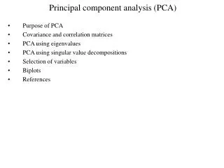
9. Principal Component Analysis (PCA) • Applications: data compression, regression, image analysis (eigenfaces), pattern recognition • Identify a linear subspace S from sample points Basis for S

10. Extensions of PCA • Probabilistic PCA (Tipping-Bishop ’99) • Identify subspace from noisy data • Gaussian noise: standard PCA • Noise in exponential family (Collins et.al ’01) • Nonlinear PCA (Scholkopf-Smola-Muller ’98) • Identify a nonlinear manifold from sample points • Embed data in a higher dimensional space and apply standard PCA • What embedding should be used? • Mixtures of PCA (Tipping-Bishop ’99) • Identify a collection of subspaces from sample points Generalized PCA (GPCA)

11. Applications of GPCA in vision and control • Geometry • Vanishing points • Image compression • Segmentation • Intensity (black-white) • Texture • Motion (2-D, 3-D) • Scene (host-guest) • Recognition • Faces (Eigenfaces) • Man - Woman • Human Gaits • Dynamic Textures • Water-steam • Biomedical imaging • Hybrid systems identification

12. Generalized Principal Component Analysis • Given points on multiple subspaces, identify • The number of subspaces and their dimensions • A basis for each subspace • The segmentation of the data points • “Chicken-and-egg” problem • Given segmentation, estimate subspaces • Given subspaces, segment the data • Prior work • Iterative algorithms: K-subspace (Ho et al. ’03), RANSAC, subspace selection and growing (Leonardis et al. ’02) • Probabilistic approaches learn the parameters of a mixture model using e.g. EM (Tipping-Bishop ‘99): • Initialization? • Geometric approaches: 2 planes in R3 (Shizawa-Maze ’91) • Factorization approaches: independent, orthogonal subspaces of equal dimension (Boult-Brown ‘91, Costeira-Kanade ‘98, Kanatani ’01)

13. Our approach to segmentation: GPCA • Towards an analytic solution to segmentation • Can we estimate ALL models simultaneously using ALL data? • When can we do so analytically? In closed form? • Is there a formula for the number of models? • We consider the most general case • Subspaces of unknown and possibly different dimensions • Subspaces may intersect arbitrarily (not only at the origin) • Subspaces do not need to be orthogonal • We propose an algebraic geometric approach to data segmentation • Number of subspaces =degree of a polynomial • Subspace basis =derivatives of a polynomial • Subspace clustering is algebraically equivalent to • Polynomial fitting • Polynomial differentiation

14. Number of groups? Introductory example: algebraic clustering in 1D

15. Number of clusters Cluster centers Solution is unique if Solution is closed form if Introductory example: algebraic clustering in 1D How to compute n, c, b’s?

16. Introductory example: algebraic clustering in 2D • What about dimension 2? • What about higher dimensions? • Complex numbers in higher dimensions? • How to find roots of a polynomial of quaternions? • Instead • Project data onto one or two dimensional space • Apply same algorithm to projected data

17. Intensity-based image segmentation • Apply GPCA to vector of image intensities N=#pixels • n=3 groups • Black • Gray • White • n=3 groups • Black • Gray • White

18. Intensity-based image segmentation Black group Gray group White group 147 x 221 Time: 2 (sec) 10 (sec) 0.4 (sec)

19. Intensity-based image segmentation 1.6 (sec) 11.4 (sec) 0.3 (sec) 1.3 (sec) 7.2 (sec)

20. Intensity-based image segmentation • Polynomial factorization • is at least 8 times faster than K-means and EM • reduces execution time of K-means and EM by 40 to 50% • performs similarly or better than K-means and EM

21. Texture-based image segmentation GPCA: 24 (sec) Human

22. Texture-based image segmentation

23. Representing one subspace • One plane • One line • One subspace can be represented with • Set of linear equations • Set of polynomials of degree 1

24. Representing n subspaces • Two planes • One plane and one line • Plane: • Line: • A union of n subspaces can be represented with a set of homogeneous polynomials of degree n De Morgan’s rule

25. Veronese map Fitting polynomials to data points • Polynomials can be written linearly in terms of the vector of coefficients by using polynomial embedding • Coefficients of the polynomials can be computed from nullspace of embedded data • Solve using least squares • N = #data points

26. Polynomial Factorization Alg. (PFA) [CVPR 2003] • Find roots of polynomial of degree in one variable • Solve linear systems in variables • Solution obtained in closed form for Finding a basis for each subspace • Case of hyperplanes: • Only one polynomial • Number of subspaces • Basis are normal vectors • Problems • Computing roots may be sensitive to noise • The estimated polynomial may not perfectly factor with noisy • Cannot be applied to subspaces of different dimensions • Polynomials are estimated up to change of basis, hence they may not factor, even with perfect data

27. Finding a basis for each subspace • To learn a mixture of subspaces we just need one positive example per class Theorem: GPCA by differentiation

28. Choosing one point per subspace • With noise and outliers • Polynomials may not be a perfect union of subspaces • Normals can estimated correctly by choosing points optimally • Distance to closest subspace without knowing segmentation?

29. There are multiple polynomials fitting the data The derivative of each polynomial gives a different normal vector Can obtain a basis for the subspace by applying PCA to normal vectors Subspaces of different dimensions

30. Minimum number of points K = dimension of ambient space n = number of subspaces In practice the dimension of each subspace ki is much smaller than K Number and dimension of the subspaces is preserved by a linear projection onto a subspace of dimension Can remove outliers by robustly fitting the subspace Open problem: how to choose projection? PCA? Dealing with high-dimensional data Subspace 1 Subspace 2

31. GPCA: Algorithm summary • Apply polynomial embedding to projected data • Obtain multiple subspace model by polynomial fitting • Solve to obtain • Need to know number of subspaces • Obtain bases & dimensions by polynomial differentiation • Optimally choose one point per subspace using distance

32. GPCA with spectral clustering • Spectral clustering • Build a similarity matrix between pairs of points • Use eigenvectors to cluster data • How to define a similarity for subspaces? • Want points in the same subspace to be close • Want points in different subspaces to be far • Use GPCA to get basis • Distance: subspace angles

33. Comparison of PFA, PDA, K-sub, EM

34. Apply GPCA in homoge-neous coordinates ( ) n=3 subspaces dimensions 3, 2 and 2 Yale Face Database B n = 3 faces N = 64 views per face K = 30x40 pixels per face Apply PCA to obtain 3 principal components Face clustering under varying illumination

35. Summary • GPCA: algorithm for clustering subspaces • Deals with unknown and possibly different dimensions • Deals with arbitrary intersections among the subspaces • Our approach is based on • Projecting data onto a low-dimensional subspace • Fittingpolynomials to projected subspaces • Differentiating polynomials to obtain a basis • Applications in image processing and computer vision • Image segmentation: intensity and texture • Image compression • Face recognition under varying illumination

36. Part IIReconstruction of Dynamic Scenes René Vidal Center for Imaging Science Johns Hopkins University

37. Structure and motion recovery • Input: Corresponding points in multiple images • Output: camera motion, scene structure, camera calibration Structure = 3D surface Motion = camera position and orientation

38. A static scene: multiple 2-D motion models A dynamic scene: multiple 3-D motion models 2-D and 3-D motion segmentation • Given an image sequence, determine • Number of motion models (affine, Euclidean, etc.) • Motion model: affine (2-D) or Euclidean (3-D) • Segmentation: model to which each pixel belongs

39. Local methods (Wang-Adelson ’94) One model per window + Kmeans Aperture, motion across boundaries Global methods (Irani-Peleg ‘92) Dominant motion: fit one motion model to all pixels Look for misaligned pixels & fit a new model to them Prior work on 2-D motion segmentation • Probabilistic approaches (Jepson-Black’93, Ayer-Sawhney ’95, Darrel-Pentland’95, Weiss-Adelson’96, Weiss’97, Torr-Szeliski-Anandan ’99) • Generative model: data membership + motion model • Obtain motion models using Expectation Maximization • E-step: Given motion models, segment image data • M-step: Given data segmentation, estimate motion models • How to initialize iterative algorithms? • Spectral clustering: normalized cuts (Shi-Malik ‘98) • Similarity matrix based on motion profile

40. Prior work on 3-D motion segmentation • Affine cameras, multiple views • Factorization methods: (Costeira-Kanade’98, Gear’98, Han-Kanade ’01, Kanatani ’01-02, Han-Kanade ‘00) • Perspective cameras (statistical approaches) • Motion segmentation & model selection (Torr’98) • Multiple rigid motions using NCuts+EM (Feng-Perona ’98) • Perspective cameras (geometric approaches) • Points in a line (Shashua-Levin ‘01) • Points in a plane moving linearly at constant speed • Points in moving in planes (Sturm ’02) • Segmentation of two rigid motions (Wolf-Shashua ‘01)

41. Data: point correspondences • Given point correspondences in multiple views, estimate • Number of motion models • Motion models: affine, projective, fundamental matrices, etc. • Segmentation: motion model associated which each • Mathematics of the problem depends on • Number of frames (2, 3, multiple) • Projection model (affine, perspective) • Motion model (affine, translational, planar motion, rigid motion) • 3-D structure (planar or not)

42. Aunifiedapproachtomotionsegmentation • Estimation of multiple motion models equivalent to estimation of onemultibody motion model • Eliminate feature clustering: multiplication • Estimate a single multibody motion model: polynomial fitting • Segment multibody motion model:polynomial differentiation chicken-and-egg

43. Aunifiedapproachtomotionsegmentation • Applies to most motion models in computer vision • All motion models can be segmented algebraically by • Fitting multibody model: real or complex polynomial to all data • Fitting individual model: differentiate polynomial at a data point

44. Segmentation of 2-D translational motions • Scene having multiple optical flows • Brightness constancy constraint (BCC) gives GPCA problem with K=3 • Multibody brightness constancy constraint

45. Segmentation of 2-D translational motions

46. Multiple epipoles (translation) Epipolar constraint: plane in Plane normal = epipoles Data = epipolar lines Multibody epipolar constraint Epipoles are derivatives of at epipolar lines Segmentation of 3-D translational motions

47. Segmentation of 3-D translational motions

48. Multibody epipolar constraint Segmentation of 3-D fundamental matrices • Rotation: • Translation: • Epipolar constraint • Multiple motions

49. Multibody epipolar constraint Multibody fundamental matrix Epipolar lines:derivatives of at a correspondence Epipoles are derivatives of at epipolar lines Fundamental matrices Segmentation of 3-D fundamental matrices

50. Segmentation of 3-D trifocal tensors • Trilinear constraint when correspond • Multibody trilinear constraint and trifocal tensor