Download
1 / 28
280 likes | 448 Vues
Chapter 9 – Tree Decomposition Methods. Anagh Lal CSCE 990-06 Advanced Constraint Processing. Outline. Acyclic constraint networks Hypergraph, dual graph, primal graph, join-tree, hypertree, acyclic constraint network. Solving acyclic constraint networks (DB ) Algorithm Acyclic-Solving

E N D
Chapter 9 – Tree Decomposition Methods Anagh Lal CSCE 990-06 Advanced Constraint Processing 1
Outline • Acyclic constraint networks • Hypergraph, dual graph, primal graph, join-tree, hypertree, acyclic constraint network. • Solving acyclic constraint networks (DB ) • Algorithm Acyclic-Solving • Identifying acyclic constraint networks • Dual-based approach • Primal-based approach • Join-tree clustering: general CSP acyclic CSP 2
Introduction • Chapter 4: tree-shaped binary CSPs can be processed efficiently • Here, the notion of a constraint tree is extended to non-binary constraints A new class: acyclic constraint networks • Review: • hypergraph • dual of a graph • primal graph 3
Examples on the board • Hypergraph • Dual graph • Reduced dual graph (when tree join-tree) • Primal graph 4
Connectedness property • An arc subgraph of a graph contains • all the nodes and • a subset of the edges • Two nodes that share variables are connected a path along which each arc contains the shared variables • An arc subgraph of the dual satisfies the connectedness property all nodes that share a variable are connected The arc subgraph is a join-graph • Connectedness the running intersection property 5
Constraint Network: R Has A Hypergraph: H Has A Dual of H: Hdual Has A Arc subgraph of Hdual: G Does G Satisfy Connectedness? G is a Join-graph Yes Is G a Tree? G is a Join-tree H is a Hyper-tree R is an Acyclic network Yes 6
Solving acyclic problems • An acyclic constraint network can be solved efficiently since its dual graph is a treeof binary constraints. • Algorithm Acyclic-Solving • is tree-based (using directional arc-consistency) • solves acyclic problems • Domains of variables in the dual problem constraint tuples of the original problem • Acyclic-Solving assumes that any tuples are consistent with domains (Relational arc-consistent) 7
Algorithm Acyclic-Solving • Input: • Acyclic constraint network R = (X, D, C) • A join-tree T of R. • Assumes the network is relational arc-consistent • Output: • (Global) consistency of network [Yes/No] • A consistent solution to R 8
Acyclic-Solving: 3 steps • Step 1: Generate an ordering d = (R1…Rt) of the constraints C such that the every constraint/relation appears before its descendants in the join-tree rooted at R1. • Step 2 (tighten relations): • Pick a relation Rj from the join-tree in reverse order of d • For each edge such that the edge connects Rj and a relation Rk that comes earlier in the ordering: • Perform a join of the two relations, project the result using the scope of the relation Rk • Assign the result of above computation to Rk (i.e., update Rk) • If Rk becomes empty: Return with no solution 9
Acyclic-Solving (cont.) • Step 3: If we reach this step, then problem is consistent. So, generate a solution. • Pick up the first relation using the ordering d. • Select a tuple from it. • Using this instantiation instantiate values from other relations such that they are consistent with previous assignments • .. And you’re guaranteed to finish! 10
Acyclic-Solving: Correctness • Step 2 of the algorithm is essentially applying directional arc-consistency along the join-tree of the dual of a problem. • As we saw in Chapter 4, this guarantees a solution for a tree network. 11
Acyclic-Solving: Complexity • Complexity of tree algorithms is O(nk2) • n: #variables • k: domain size • Expected complexity is O(rl2) • r: #constraints • each with most l tuples • Using lexicographical sorting complexity down to O(r.l.log l) 12
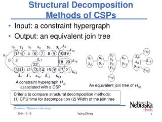
Recognizing acyclic networks Two methods • Dual-Acyclicity: dual-based recognition • Generates ‘maximal’ spanning tree of dual graph • Tests for connectedness of this spanning tree • Primal-Acyclicity: primal-based recognition • Uses the fact that the primal graph for a hypertree must be chordal 13
Dual-Acyclicity • Input: Hypergraph H of constraint network R(X, D, C) • Output: A join-tree T(S, E) if R is acyclic • Algorithm: • Generate a maximal spanning tree T of the dual of R (weight = number of shared variables) • For every two nodes u and v in T, do • If the unique path connecting them does not satisfy the connectedness property, then Exit (R is not acyclic) • R is acyclic, and T is the join-tree 14
Dual-Acyclicity: complexity • O(e3), where e is the number of constraints 15
Refresher of Chapter 4 • Maximal cardinality ordering • Chordal graph • A graph is chordal if, in a maximum cardinality ordering, each node’s parents are connected • Finding max-cliques in chordal graphs can be done in linear time 16
Primal-Acyclicity: principle • Uses 2 tests • the primal graph G of the network is chordal and • the max-cliques of the chordal primal graph G satisfies the conformatlity property • Conformality • A chordal primal graph is conformal relative to a constraint hypergraph there is a 1-to-1 mapping between maximal cliques and scopes of constraints 17
Primal-Acyclicity • Input: A network R = (X, D, C) and its primal graph G • Output: A join-tree iff the problem is acyclic • Algorithm: 3 steps • Test chordality of the primal graph G • Test conformality of the primal graph G • If acyclicity, then create the join-tree for R 18
Primal-acyclicity: the steps • Test chordality: Using a max-cardinality ordering d of G and starting from the last node check if the parents of all the nodes are connected. If for any node they are not then, exit: problem is not acyclic • Test conformality: Let C1,…,Ctbe the cliques indexed by their highest variable in the ordering. Check if the cliques correspond to scopes of constraints, if so R is acyclic • Create a join-tree: From t to 1, connect every clique to an earlier clique with which it shares a maximal number of variables Return the tree of cliques 19
Join-tree clustering • Since acyclic constraint networks can be solved efficiently, try to convert an arbitrary constraint network into an acyclic one • This can be achieved by grouping subsets of constraints into clusters, or sub-problems, whose scopes constitute a hypertree, thus transforming a constraint hypergraph into a constraint hypertree • By replacing each sub-problem with its solution we obtain an acyclic constraint problem, which can be solved using the acyclic solving algorithm. • This compilation process is called join-tree clustering 20
Hypertree embedding • A hypertree embedding of a hypergraph R = (X,H) is a hypertree T = (X,S) such that, for every h element of H there is a h1 element of S such that h is a subset of h1. 22
Decomposing a hypergraph into a hypertree • Consider the primal-acyclicity algorithm to detect acyclic networks. Instead of terminating when we find that the graph is acyclic we could repair the primal graph and proceed to convert the hypergraph to a hypertree. • Enforce chordality by connecting the parents • Enforce conformality by generating unique constraint for every maximal clique. • Algorithm Join Tree Clustering (JTC) does this. 23
Joint Tree Clustering • Input: Constraint problem R = (X, D, C) and its primal graph G = (X, E) • Output: An equivalent acyclic problem and its join-tree: T=(X, D, C’) 24
JTC algorithm (cont.) • Select a variable ordering d (max-cardinality recommended) • Triangulation: Connect the parents. Generate an induced graph along d. • Create a join-tree for the induced graph • Identify all max cliques in the chordal graph. (C1,…,Ct), from the last variable to the first. • Connect each Ci to one single Cj (j < i) with whom it shares the largest subset of variables. 25
JTC algorithm (cont.) • Place each constraint from R in one clique containing its scope, and let Pi be the constraint subproblem associated with Ci • Solve each Pi and let R’i be its set of solutions • Return C’ = {R’1,…, R’t}, and their join-tree, T 26
Complexity • Time and space complexity: • O(r.k(w*(d)+1)) 27
Discussion • Questions? • Comments? 28