Download
1 / 24
250 likes | 264 Vues
Introduction to Multiple Linear Regression in SPSS. Jennifer Williams March 9 th , 2019. Hello!. Who am I? Why are we here? What’s the point of it all?. When to Use SPSS. Note the name: Statistical Package for the Social Sciences

E N D
Introduction to Multiple Linear Regression in SPSS Jennifer Williams March 9th, 2019
Hello! • Who am I? • Why are we here? • What’s the point of it all?
When to Use SPSS • Note the name:Statistical Package for the Social Sciences • SPSS has many uses, but it was designed for research. It is being adapted for more business and marketing analyses, as well. • Hi, Accounting students! You’re welcome here, but you’ll definitely want to get friendly with Excel. • SPSS is frequently used for descriptive and inferential statistics. (Remember these from the first chapter of your stats class?) • Guys?
Some Context • We want to make decisions about what is likely true in general, but we can only collect so much information. How do we use the information we’ve collected (our sample) to make generalizations about everyone (our population)? This is the “point” of the field of statistics. • We frequently use measures of central tendency and spread to summarize our data and make inferences about the population. • Mean: the sum of all data points, divided by your sample size. The “average.” Often our “best guess.” • Standard deviation: basically, the average deviation from the mean, aka how far scores tend to fall from the mean.
More Context (It’s Important) • Frequently, we want to make generalizations and predictions about certain outcomes that are quantitative in nature. • Examples: • Income Level • Ice Cream Purchased in a Year • Sales of a Product at a Certain Store • You have a few options here, based on the type of data you have and the outcome variable you wish to understand. • Moving averages: Base your estimates of future performance on past performance of that same variable. • Regression: Base your estimates of future performance on information from other predictor variables.
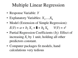
What is linear regression? • Linear regression uses the least-squares method to find a straight line that predicts an outcome variable (ŷ) based on scores on predictor variable(s). • Linear equation: • ŷ = b0 + b1x1 + … + bnxn • Meaning of Slopes • Meaning of y-intercept
When to use linear regression • You can have as many predictor variables as you’d like (within reason*). They can be categorical or continuous. Your outcome variable (also called response variable) must be quantitative. • Seriously. Must be quantitative. Rookie mistake. • Your data must meet certain criteria or assumptions, which you can generally test in SPSS. • Regression analysis has two main components: • Hypothesis Testing (Is this model any good?) • Prediction (What does this model tell me to expect?) *Typically, statisticians recommend 10-20 observations per variable.
Hypothesis Testing Review • In statistics, we start with a certain model, called the Null Hypothesis, AKA the nope hypothesis. • We stick to this Null Hypothesis unless we have strong evidence that it is unreasonable to do so. When the Null Hypothesis seems unreasonable enough,* we reject it. • We then collect sample information and calculate the probability of finding that information, given the assumption that the Null Hypothesis is true. This probability is called a p-value. • *We set a threshold, called alpha, which is our cutoff for determining when to reject the Null Hypothesis in favor of the Alternative Hypothesis. • We generally use an alpha of .05.
What *can* linear regression tell us? • Strength of Overall Model • Hypothesis tests, model diagnostics • Strength of Individual Predictors • Hypothesis tests, slopes (aka b-weights) • Predicted Values Based on Model • Plug it in
What *can’t* linear regression tell us? Correlation/regression caustion.
Assumptions of Linear Regression • Linearity • Scatterplots • Residual Plot • No outliers/influential data points • Boxplots/Histograms • Diagnostics • Normality • Histogram • Explore • The Central Limit Theorem • Homoscedasticity (consistency) of residuals • Residual Plot • No multicollinearity • Regression Diagnostics • Independence of observations • Regression Diagnostics • Your Noggins* *You can’t math your way out of bad methods!
Let’s Dig In! Time to Open Your SPSS File. • Lending Club data from loans originated between 2007 & 2011. All are either charged off or paid off. • Different types of SPSS files: • Data: .sav • Output: .spvSyntax: .sps • Hitting “Paste” during point-and-click navigation will send code to the Syntax window. • Data File Views: • Variable view • Name • Type • Label • Values • Missing • Measure • Data view
Our Variables • Our Response Variable: Percentage of Original Repaid • Transform -> Compute Variable • Our Predictor Variables: • Loan Grade (3 Categories) • DTI (Debt to Income Ratio) • Categorical Variables Require “Dummy Coding.” • Select a category to serve as the “reference category” aka baseline. • Assign 0’s and 1’s to the different groups; the total number of dummy variables = # of groups - 1 • Transform -> Recode into Different Variables* • If you have quite a few dummy variables to make, use the “Paste” button to open Syntax, then copy and paste to save some time. *I almost always recode into different variables, so my original data remain in my file.
More on Dummy Coding • Slopes tell us how much we expect a person’s score to change if their predictor score increases by one point. • For categorical variables, there are no “points,” so we build categories into the equation by creating different terms for the categories. • We choose a reference group to be the “baseline;” they’ll have a score of 0 on all terms related to this variable. The regression equation will tell us, at baseline, what we expect when every predictor is zero. This gives us the score we expect when a person has a zero on quantitative predictors AND belongs to the reference group.
Data Cleaning & Assumption Checking • First, let’s examine DTI and Percentage Repaid for distribution & outliers. • Analyze -> Descriptive Statistics -> Explore. Move variable of interest to “Dependent List Click “Statistics” then “Outliers.” Click “Plots,” select “Histogram” and uncheck “Stem and Leaf” • DTI looks great. Really symmetrical. Percentage Repaid… Has great personality? • A few options: • Trimming • Transforming, especially Logarithmic (positive skew) or Exponential (negative skew). • Next, check scatterplots of relationships between outcome and any quantitative predictors. • Graphs -> Legacy Dialogs -> Scatter/Dot
Linear Regression Procedure • Analyze -> Regression -> Linear • Leave Method Set to “Enter.” Move a block of variables over; if using multiple blocks, hit “next” to move to a new block. Order is important when using blocks! • Click Statistics. Select Estimates, Model Fit, R Squared Change, Descriptives, Collinearity Diagnostics • Click Plots, select *Zresidfor the Y-axis and *Zpredfor the X-axis. Also select Histogram and Normal Probability Plot.
Output Organization • Descriptives • Useful for mean, standard deviation, and sample size. Watch out for categorical & transformed predictors, though! • Correlations • Bivariate correlations among all predictors and the response. • Model Summary • Overview of how well model fits the data • ANOVA • Test of overall model. The gatekeeper! • Coefficients • Tests of individual predictors. Only check this if ANOVA is significant! • Collinearity Diagnostics • Residuals Statistics • Tests of influential cases • Charts • Histogram – Normality of residuals • PP Plot – Normality of Residuals • Residuals Plot - Homoscedasticity
Interpreting Regression Output: Assumptions • Independence: Durbin-Watson checks for autocorrelation (lack of independence). Varies between 0-4, with 2 meaning residuals are uncorrelated. Values <1 and >3 are cause for concern. • Collinearity: VIF > 10 considered a problem; these variables would be too highly correlated for provide a stable model. • Influential cases: • Cook’s measures overall influence on model. Values >1 cause for concern. • Average Leverage, another measure of potential influence, is calculated as (k+1)/n . Values 2 or 3 times this size are problematic. • Mahalanobis Distance, also related to leverage, follows chi-squared distribution, with df = k, where k = number of predictors. You can use this to identify a critical value. • To identify problematic cases, use Analyze -> Reports -> Case Summaries. Be sure to show case numbers and to deselect option to limit cases shown. • To exclude problematic cases, use Data -> Select Cases -> If Condition is Satisfied.
Interpreting Regression Output: More Assumptions • Normality of Residuals: • Regression is fairly robust to violations of normality of residuals, as long as the sample size is adequate. • Check histograms and normal PP plots; if working with a small sample size, consider a transformation. • Homoscedasticity of Residuals: • Check those residual plots. They should look like a random ink spray. (Watch out for categorical predictors, though. They’ll create vertical lines in the graph.)
Interpreting Regression Outputs: The Model • Multiple R: Always positive, shows the relationship between your model (prediction) and your outcome variable. Higher values indicate greater prediction accuracy. • R2: Variance in your outcome variable explained by your model. • R2 change: Additional variance accounted for by the introduction of the new block of variables. Only useful when using blocks. • ANOVA: A hypothesis test based on the null hypothesis that your model offers no better prediction of outcome variable than simply using the average of the outcome variable. • A p-value <.05 indicates that at least one predictor is significant, usually.
Interpreting Regression Outputs: Individual Predictors • B-weights: • Predictors: How much the predicted response will change per unit increase in the predictor variable, when all other variables are held constant. AKA, slopes. • Constant: The predicted value of the outcome variable when the value of ALL predictors is 0. AKA, y-intercept. • SE: Standard error of the b-weight, a measure of how much these coefficients are likely to vary from the population value in different samples. • Beta-weight: A standardized coefficient, showing how many standard deviations the predicted response will change per standard deviation increase in the predictor variable, when all other variables are held constant. • T-test & p-values: Test of the null hypothesis that the b-weights are equal to zero (signifying no relationship).
Your Turn! • Select two predictor variables. • For quantitative variables, check distribution shape and outliers. • Conduct a linear regression analysis predicting percentage of loan payoff from those two variables. Follow the same procedure as described in these slides. • Does a regression analysis appear to be a good fit for these data, based on the assumptions you’ve checked? • In particular, pay attention to residual plots! • Does your overall model appear to predict percentage of loan payoff? If so, move to next question. • How well does each predictor predict percentage of loan payoff? • Is it a significant predictor? • How much does predicted percentage of loan payoff change if you increase the predictor score by one unit?
Conclusion • Linear regression is a powerful tool and one of the most commonly used statistical techniques out there. Your employers will expect you to be familiar with it. • Watch out for overstating the conclusions you can draw from your analyses. • Make sure that your data are a good fit for the model you use. • Regression can help you predict performance based on information about other variables. It can also give you information about which variables are most important to collect information about. • Search out manuals that are easy to use and understand, and keep them close. You don’t need to memorize this information; you need to understand it well enough to replicate it with help.
Recommended Resources • Field, A. (2013). Discovering statistics using IBM SPSS Statistics. Los Angeles: Sage. • In general, Andy Field is a great resource for using SPSS. Look him up on YouTube! • Laerd.com offers many great tutorials, though there is a fee. • Stattrek.com is often very helpful, though less detailed. It’s free, though!