Download
1 / 27
270 likes | 273 Vues
Learn about the implementation of the Local Ensemble Kalman Filter on the NCEP Global Forecast System (GFS) and its advantages for data assimilation. Discover the concepts, extensions, and future plans of the LEKF. Presented by the Chaos-Weather Team at the University of Maryland College Park.

E N D
Implementation of the LEKF on the NCEP GFS: “Perfect Model” Experiments Chaos-Weather Team University of Maryland College Park Camp Springs, MD, February 27, 2004
UMCP Chaos-Weather Team Founders: E. Kalnay and J. Yorke Theory: B. Hunt and E. Ott et al. 4D Extension: B. Hunt, T. Sauer, and J. Yorke et al. GFS Implementation: I. Szunyogh, E. Kostelich and G. Gyarmati et al. An interdisciplinary team of experts in dynamical systems theory, meteorology, mathematics, and scientific computing
Outline • The LEKF Concept • 4-D Extension • Implementation on the NCEP GFS • Conclusions • Future Plans
Data Assimilation Observation pdf Analysis pdf For the Grid Initial Condition: Analysis Mean t3 Forecast pdf For the Grid t1 t2 Kalman Filter: The analysis uncertainty is evolved using the model dynamics to obtain the forecast uncertainty
Ensemble Kalman Filtering Ensemble of Initial conditions Background Ensemble t1 t2 • Ensemble Kalman Filters (EnKF):(i) Multiple analyses are prepared, and then (ii) the most likely state is determined by the mean of the analysis ensemble • Ensemble Square-root Filters (EnSF):(ii) The most likely state is determined first, and then (ii) the mean state is perturbed to obtain the analysis ensemble
Examples • EnKF: Evensen (1994), Houtekamer and Mitchell (1998, 2001), Hamill and Snyder (2000), Anderson and Anderson (1999), Keppene and Rienecker (2002) • EnSF: Anderson (2001), Bishop et al. (2001), Whitaker and Hamill (2002), Tippett et al. (2002), LEKF (Ott et al., 2003a, b) • What is the difference between our scheme and other square-root filters? The LEKF is not a sequential data assimilation scheme.
Sequential Schemes • The observations are assimilated sequentially • A local region around the grid point is defined by the Gaussian filter of Gaspari and Cohn (1998) • The state estimate is updated at all grid-points within the local region
Local Ensemble Kalman Filter • The state estimate is updated concurrently at the different grid-points • A local region is defined (the shape is arbitrary, no forced distance dependent reduction of the correlation) • All observations within the local region are assimilated
Potential Advantages of the LEKF • Allows for significant reduction of the dimension, based on estimating the complexity of the dynamics (efficient filtering of redundant information from the observations) • Efficient for observations with correlated errors • The computation can be performed concurrently for each grid point • We believe that this formulation is advantageous, when many observations, especially those with correlated errors, are assimilated
Potential Disadvantages of the LEKF • When the observations are sparse (when the local regions must be large) the Gaussian filter may be a better tool to localize the covariance information (more efficient filtering of spurious long distance correlations) • When the number of observations is significantly lower than the number of grid points, the LEKF is probably more expensive than a sequential scheme • We expect that sequential schemes are more suitable than the LEKF, when relatively few observations are assimilated (e.g.; Whitaker et al. 2003: Reanalysis without radio-sondes …)
Schematic of the LEKF Analysis ensemble at t-1 Evolve model from t-1 to t Global analysis ensemble at t Background ensemble at t Obtain Global Analysis Ensemble … Form local vectors Local Analysis Ensembles Local background vectors Local analysis and Analysis Error covariance matrix Do local analysis Obtain Local Analysis Ensembles
Illustration by the Lorenz-96 model Unstable non-linear waves with a typical wavelength of 5-6 grid points (the wavelength is independent of the M) xM=x1 xM-1 x2 x3 “Eastward group velocity” For M=40 the Lyapunov dimension is 27.1 Prototype of a spatio-temporally chaotic system with a finite correlation length
LEKF vs. Global EKF Global • The global scheme requires an increasing number of ensemble members as the size of the system increases • The number of ensemble members needed in the LEKF is much lower than in the global scheme and independent of the system size M=40 ~Lyapunov dimension M=80 M=120 Local
4D Ensemble Kalman Filter Hunt et. al 2004a,b: Ensemble Kalman Filters allow for assimilating observations at the correct time: y=h(x) model state observation observational operator xb=Ebe background mean background ensemble vector of linear weights H’ does not exist for a single background y-Hxo=y-HEoe=y-H’xb innovation at obs. time ensemble at obs. time modified H
4D Ensemble Kalman Filter Illustration by the 40-variable Lorenz model Approach used in 3D-Var Schemes Only data at analysis Times are used 4D Ens. KF
NCEP GFS • A time series of “true states” is generated by a long integration of the model started from the operational NCEP analysis at January 1, 2000. • The ”observations” are created by adding Gaussian random noise to the true state(the errors:1 Kfor temperature,1.1 m/sfor wind vector components, and1 hPafor surface pressure) • The lower boundary condition of an analysis ensemble member is copied from the associated background ensemble member • The simulated observations are assimilated and the result is compared to the `true state’ • This experimental design allows fortesting our fundamental hypothesis, that the local dimensionality of the model is low (whether we can stay close to the true state by estimating the state in local low-dimensional spaces) • This is a crucial step, which is needed for us to be able to distinguish between problems in our formulation (and implementation) and the effects of model errors
Experiments • Red (“Base Line”): 80-member, the surface pressure, temperature and wind are observed at each grid point, ozone and humidity copied from “truth” • Green: Same as Red, except 40-members and 90% of the observations are removed • Dark Blue: Same as Red, except 40-members are removed, and ozone and humidity are copied from background • Light Blue (“Realistic”): Same as Red, except 40 members and 90% of the observations are removed, ozone and humidity are copied from background
Similarly good convergence was Also found for the other variables All implementations are Close to the “Base line” Observational error
Conclusions • While some modest improvement is expected from further tuning parameters in the “Perfect Model” environment, the LEKF is ready for testing with real observations • Based on the “Perfect Model” experiments it is expected that the LEKF analyses will have the highest quality in the extra-tropic (where a modest size ensemble, and a modest number of observations are sufficient), while analyses in the Tropics will improve with increased observational density. Some modest improvement can be expected when the ensemble size is increased
“Near Future” Work • Implementation of the 4D extension (in progress) • Assimilation of radiosonde observations (in progress) • Implementation on the NCEP RSM (in progress) • Surface Analysis (your help is wanted!) • Implementation on the NASA model (starts soon) • Handling of model errors (in the theoretical phase) • Direct minimization of the cost function (in the theoretical phase)