Download
1 / 6
60 likes | 625 Vues
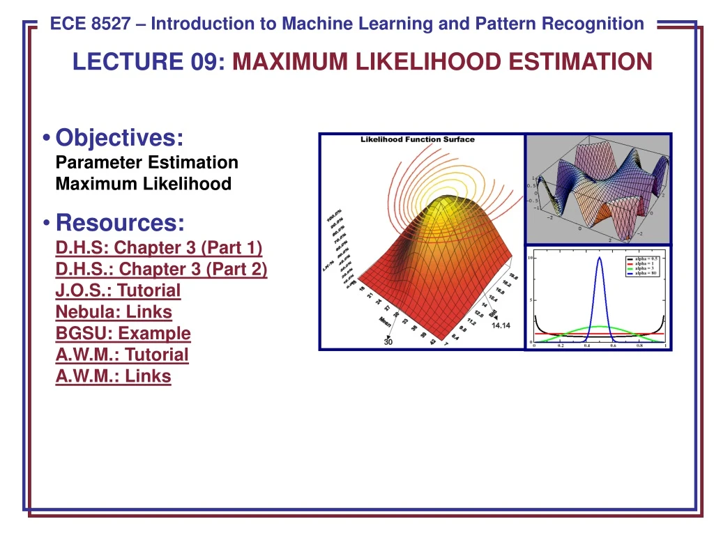
LECTURE 09: MAXIMUM LIKELIHOOD ESTIMATION. • Objectives: Parameter Estimation Maximum Likelihood Resources: D.H.S: Chapter 3 (Part 1) D.H.S.: Chapter 3 (Part 2) J.O.S.: Tutorial Nebula: Links BGSU: Example A.W.M.: Tutorial A.W.M .: Links. Introduction to Maximum Likelihood Estimation.

E N D
LECTURE 09: MAXIMUM LIKELIHOOD ESTIMATION • • Objectives:Parameter EstimationMaximum Likelihood • Resources:D.H.S: Chapter 3 (Part 1)D.H.S.: Chapter 3 (Part 2)J.O.S.: TutorialNebula: LinksBGSU: ExampleA.W.M.: TutorialA.W.M.: Links
Introduction to Maximum Likelihood Estimation • In Chapter 2, we learned how to design an optimal classifier if we knew the prior probabilities, P(ωi), and class-conditional densities, p(x|ωi). • What can we do if we do not have this information? • What limitations do we face? • There are two common approaches to parameter estimation: maximum likelihood and Bayesian estimation. • Maximum Likelihood: treat the parameters as quantities whose values are fixed but unknown. • Bayes: treat the parameters as random variables having some known prior distribution. Observations of samples converts this to a posterior. • Bayesian Learning: sharpen the a posteriori density causing it to peak near the true value.
General Principle • I.I.D.: c data sets, D1,...,Dc, where Djdrawn independently according to p(x|ωj). • Assume p(x|ωj) has a known parametric form and is completely determined by the parameter vector θj(e.g., p(x|ωj) ~N(μj,Σj),where θj=[μ1, ..., μj,σ11,σ12, ...,σdd]). • p(x|ωj) has an explicit dependence on θj:p(x|ωj,θj) • Use training samples to estimate θ1,θ2,..., θc • Functional independence: assume Di gives no useful informationabout θjfor i≠j. • Simplifies notation to a set Dof training samples (x1,...xn) drawn independently from p(x|ω) to estimate ω. • Because the samples were drawn independently:
Example of ML Estimation • p(D|θ) is called the likelihood of θ with respect to the data. • The value of θ that maximizes this likelihood, denoted , • is the maximum likelihood estimate (ML) of θ. • Given several training points • Top: candidate source distributions are shown • Which distribution is the ML estimate? • Middle: an estimate of the likelihood of the data as a function of θ (the mean) • Bottom: log likelihood
General Mathematics • The ML estimate is found by solving this equation: • The solution to this equation can be a global maximum, a local maximum, or even an inflection point. • Under what conditions is it a global maximum?
Summary • To develop an optimal classifier, we need reliable estimates of the statistics of the features. • In Maximum Likelihood (ML) estimation, we treat the parameters as having unknown but fixed values. • Justified many well-known results for estimating parameters (e.g., computing the mean by summing the observations).