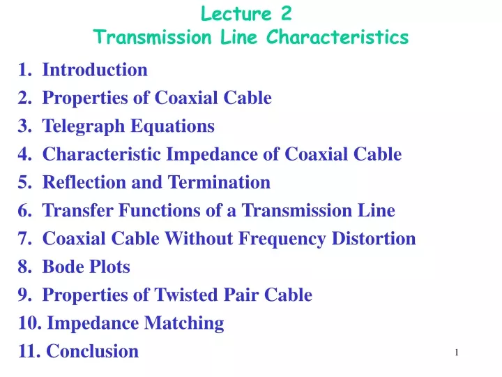
Lecture 2 Transmission Line Characteristics

1. Lecture 2 Transmission Line Characteristics 1. Introduction 2. Properties of Coaxial Cable 3. Telegraph Equations 4. Characteristic Impedance of Coaxial Cable 5. Reflection and Termination 6. Transfer Functions of a Transmission Line 7. Coaxial Cable Without Frequency Distortion 8. Bode Plots 9. Properties of Twisted Pair Cable 10. Impedance Matching 11. Conclusion

2. Introduction • A communication network is a collection of network elements integrated and managed to support the transfer of information. • Data Transmission: links and switches. • Optical fiber • Copper coaxial cable • Unshielded twisted wire pair • Microwave or radio “wireless” links. • Optical fiber and copper links are usually point-to-point links, whereas radio links are usually broadcast links. • Guided media: • twisted pair (unshielded and shielded) • coaxial cable • optical fiber • Unguided media: • radio waves • microwaves (high frequency radio waves)

4. Coaxial cable with length l. It is composed of a number of intermediate segments with properties: R, L, G and C of a unit length of cable R1: radius of inner wire R2: radius of braided outer conductor 2·10-7: derived from properties of dielectric material

5. Telegraph Equations x  0: (2) (1) Equations (1) and (2) are called the telegraph equations.

6. They determine e(x,t) and i(x,t) from the initial and the boundary conditions. • (If we set R and L to zero in these equations (we assume no series impedance), the simplified equations are telephonic equations). (3) (4) • Solution of equations (3,4) by differentiating of equation (3) with respect to x, and combine with equation (4):

7. Define the value as (5) (6) A1 and A2 are independent of x, and can be calculated from the boundary conditions at x = 0 and x = l. The value of is derived from the properties of the coaxial cable and the frequency : (7) () is the attenuation coefficient.() is the phase shift coefficient.

8. Characteristic Impedance of Coaxial Cable For the Fourier-transformed current insert (6) into equation (3) from equation (7) above:

9. Reflection and Termination reflected voltage/incident voltage; • To express this signal in the time domain, we must divide (6) into its magnitude and phase components. We express  =F(,):

10. We can find the relationship between the magnitudes of A1 and A2 if we know that Zrec is pure resistance (a real value of impedance) and we know the value of Z:

11. Z = 50, Rtot= 50, and = 2 V • Zrec = 0, • Zrec = 50 • Zrec = 

12. Ethernet Technologies: 10Base2 • 10: 10Mbps; 2: under 200 meters max cable length • thin coaxial cable in a bus topology • repeaters used to connect up to multiple segments • repeater repeats bits it hears on one interface to its other interfaces: physical layer device only!

14. Ethernet Cabling The most common kinds of Ethernet cabling.

15. Transfer Functions of Coaxial Cable For f<100 kHz

17. Bode Plots

20. Appendix • Error analysis • The goal of the lab experiment is to determination the transmission line bandwidth of a coaxial cable. We will use the experimental data to construct an amplitude Bode plot, and find the frequency for which the signal is attenuated by less than ‑3 dB. • This is the bandwidth for which half or more of the input signal power is delivered to the output. • the absolute error in 20·log10 |H(j)| due to the errors Uout and Uin :

21. transfer from decimal to natural logarithms with the correction factor 0.434 [log10(e)]: The worst case will occur when Vout = -Vin . If we set Vout = 0.025:

22. Amplitude bode plot with error bars on amplitude axis.