Download
1 / 46
480 likes | 688 Vues
The 2dF galaxy redshift survey. John Peacock & the 2dFGRS team. Harvard, October 1999. Outline. Brief history 2dF Survey motivation & design Survey data Spectral classification Results: Luminosity function Correlation function Galaxy bias & future issues. (1) Autocorrelation function.

E N D
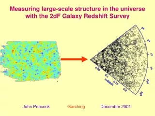
The 2dF galaxyredshift survey John Peacock & the 2dFGRS team Harvard, October 1999
Outline • Brief history • 2dF Survey motivation & design • Survey data • Spectral classification • Results: • Luminosity function • Correlation function • Galaxy bias & future issues
(1) Autocorrelation function rmass= r0(1+d)xA(r) = < d(x) d(x+r) > (2) Two-point correlations dV2 prob(pair) = <n>2 dV1 dV2 [1 + x2(r) ] dV1 r xA(r) = x2(r) ? - only if Poisson Clustering Hypothesis is true History of galaxy clustering • 1930s: Hubble lognormal cell counts • 1940s/50s: Eyeball surveys (Shane & Wirtanen, Zwicky, Abell…) • 1970s: Correlation functions
r ~ r-a (r < R) ” x ~ r-(2a-3) obs: x ~ r-1.8 ” a = 2.4? Meaning of clustering Neyman Scott & Shane (1953): random clump model Modern view: gravitational instability of (C)DM - sheets, pancakes, filaments, voids...
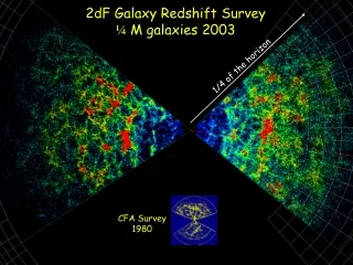
Redshift Surveys CfA/SSRS z-survey ~15000 z’s Las Campanas Redshift Survey ~25000 z’s
The 2dF Galaxy Redshift Survey • Aim for LCRS X 10 = 250,000 z’s • Increase sky coverage to get fully 3D sample • Measure >100-Mpc power • Test Gaussian nature of linear fluctuations • Measure redshift-space distortions • Increase sampling density • Spatial distribution for different galaxy types • Tests of theories for biased galaxy formation
2dFGRS Survey Team • Australian team members:Matthew Colless, Joss Bland-Hawthorn, Russell Cannon, Warrick Couch, Kathryn Deeley, Roberto De Propris, Karl Glazebrook, Carole Jackson, Ian Lewis, Bruce Peterson, Ian Price, Keith Taylor. • British team members:Steve Maddox, John Peacock, Shaun Cole, Chris Collins, Nicholas Cross, Gavin Dalton, Simon Driver, George Efstathiou, Richard Ellis, Carlos Frenk, Ofer Lahav, Stuart Lumsden, Stephen Moody, Peder Norberg, Shai Ronen, Mark Seabourne, Robert Smith, Will Sutherland, Helen Tadros.
2dFGRS parameters • Galaxies: bJ 19.45 from revised APM • Total area on sky ~ 2000 º • 250,000 galaxies in total, 93% sampling rate • Mean redshift <z> ~ 0.1, almost all with z < 0.3
2dFGRS geometry ~2000 sq.deg. 250,000 galaxies Strips+random fields ~ 1x10⁸ h-3 Mpc3 Volume in strips ~ 3x10⁷ h-3 Mpc3 NGP SGP NGP 75x7.5 SGP 75x15 Random 100x2Ø ~70,000 ~140,000 ~40,000
Tiling strategy ‘2dF’ = ‘two-degree field’ = 400 spectra Efficient sky coverage, but variable completeness High completeness through adaptive tiling: multiple coverage of high-density regions
Sampling: 2dF vs LCRS 2dFGRS (~93%) LCRS (~25%)
Recalibrated number counts Old APM counts Recalibrated APM counts
Prime Focus The 2dF site
>12 arcsec spacing; 15 degree bend <10 seconds to position each fibre Configuring fibres
Survey status - August 1999 • Observed: • 227/1093 fields • 58764 targets • 4037 repeats • Redshifts/IDs: • 53192 (91% complete) • 50180 galaxies • 2993 stars, 19 QSOs
Redshift yield • The median redshift yield is 93%. • 10% of fields have a yield less than 80%. • 30% of fields have a yield less than 90%. • After ADC s/w fix, good conditions routinely give yields >95%. • Reliability: of 1404 z’s in overlap with LCRS, only 8 disagree (99.4% agree).
Completeness • Redshift completeness is >90% for bJ<19 but drops to 80-85% at bJ=19.45. • Completeness is similar in NGP and SGP strips. • Completeness as a function of magnitude varies with the overall completeness of the field. • Selection function depends on (at least) overall completeness and magnitude.
Survey mask NGP SGP Cutouts are bright stars and satellite trails.
100% 100% 0% 0% Selection mask NGP ‘Bitten-cookie’ effect from missing overlap tiles. SGP
20% 20% 0% 0% Stellar contamination NGP Contamination by objects with z~0. SGP Typical level of stellar contamination is <5%.
At least some data were obtained on 61/99 of nights so far allocated to survey. Over all nights with any data, the mean number of fields/night is 4.5. Averaged over year, expect to get 7 fields for each completely clear night = 3000 z’s per night Full survey requires about 100 clear dark nights, or all dark time for 1 year. In practice 2dFGRS uses about 1/3 AAT dark and will take 3 years Survey rate
The big picture The 2dF galaxy + QSO redshift surveys 2dFGRS 50180 galaxies 6824 QSOs
Redshift distribution Mean redshift <z>=0.11; almost all z<0.3. N(z) still shows significant clustering.
2 fit to 1/Vmax LF STY Schechter fit gives a -1.2 (due to clustering? non-Schechter form?) Small numbers at MB>-14. Overall luminosity function (mean K-corrections)
Early PC3 Early PC2 Late PC1 Late Mean spectrum Spectral classification by PCA • Apply Principal Component analysis to spectra. • PC1: emission lines correlate with blue continuum. • PC2: strength of emission lines without continuum. • PC3: strength of Balmer lines w.r.t. other emission. • Classify spectral types in PC1-PC2 plane using sample of Kennicutt to set bounds. • Further work: • effect of spectro-photometric errors; • self-classification algorithms; • calibration against spectral models.
1/Vmax LF Sum of Schechter fits to each type STY fit Overall STY Schechter fit Early a All Late M* LFs by spectral type • For 12,000 galaxies with PCA types, fit LFs by type. • 1/Vmax LFs have less-steep faint ends than STY fits of Schechter functions. • From early to late types… • M* gets fainter: -19.6 -18.9 • gets steeper: -0.7 -1.7 • Overall M* brighter than M* of any type; Schechter function not adequate fit. • Evidence for upturn at faint end of LF.
Early types (1,2) Late types (3,4,5) Galaxy distribution by type
r s p 2D correlations x(s, p)
Model comparison - I Flattening depends on b=W0.6/b (dgal = b dmass) Fingers of God infall
Model comparison - II Analyze x(s,p) into Legendre polynomials: get b from quadrupole-to-monopole ratio -P2/P0 = (4b/3 + 4b2/7) / (1 + 2b/3 + b2/5) Linear Damping by fingers of God
Projected correlations X(r) APM w(q) deprojection works well to r = 20 h-1 Mpc (cosmic variance matters on larger scales)
The CDM clustering problem Non-monotonic scale-dependent bias LCDM tCDM b2 = xg / xm Jenkins et al. 1998 ApJ 499, 20
Numerical galaxy formation Durham Munich Santa Cruz Edinburgh ...
Antibias in LCDM Benson et al. astro-ph/9903343
Dark-matter haloes and bias Moore et al: r = [ y3/2(1+y3/2) ]-1; y = r/rc
Correlations from smooth haloes LCDM NL APM Lin tCDM PS++ mass function and NFW++ halo profile gives correct clustering
Halo occupations depend on mass PS++ mass function wrong shape for cluster/group LF LCDM Correct weighting of low-mass haloes predicts antibias
Summary • 2dF survey status • Over 50,000 redshifts (20% of survey) • Expect 100,000 March 2000 • 250,000 March 2001 • Preliminary results • Luminosity functions by spectral type • Correlations and redshift-space distortions • Future issues • Clustering on 100-Mpc scales • Gaussian nature of density field • Clustering by spectral type and luminosity • Detailed tests of halo-based bias models