Download
1 / 11
110 likes | 183 Vues
CS164: 2D and 3D Transformations. Leonidas Guibas Computer Science Dept. Stanford University. Kronecker conditioning experiments. Experiment setup: Simulate some # of mixings followed by a single observation

E N D
CS164: 2D and 3D Transformations Leonidas Guibas Computer Science Dept. Stanford University
Kronecker conditioning experiments • Experiment setup: • Simulate some # of mixings followed by a single observation • Use bandlimited Fourier domain algorithms to infer posterior distribution after observation • Validation: • Measure the L1 error between approximation and true distribution
Kronecker Conditioning experiments Error of Kronecker Conditioning, n=8 (as a function of diffuseness) 1st order 0.1 2nd order unordered 2nd order ordered 0.08 0.06 Better error (averaged over 10 runs) 0.04 0.02 1 L 0 0 5 10 15 # Mixing Events Measured at 1st order marginals (Keeping 3rd order marginals is enough to ensure zero error for 1st order marginals)
Simulated data drawn from model • Experiment setup: • Observation sequence (250 timeslices) simulated from hidden Markov model (n=6) • Used Fourier domain algorithms to approximately infer distribution over hidden states • Validation: • Average (L1) error between approximation and true distribution
HMM simulation results Projection to the Marginal polytope versus no projection 0.12 Without Projection 0.1 0.08 1st order error at 1st order Marginals With Projection Averaged over 250 timesteps Better 0.06 2nd order 3rd order 0.04 0.02 1 L 0 1st order 2nd order 3rd order Approximation by a uniform distribution
Tracking with a camera network • Experiment setup: • Stanford camera network dataset • 8 cameras, multiple views, occlusion effects • N=11 individuals walking in lab environment • Observation models based on color histograms • Mixing events declared when 1.) two people walk close to each other, 2.) among everyone outside of the room • Validation: • Average number of tracks correctly identified
Tracking results Omniscient tracker 60 50 40 Better % Tracks correctly Identified 30 20 10 0 clip from data time-independent classification w/o Projection with Projection
Scaling • For fixed representation depth, Fourier domain inference is polytime: • But complexity can still be bad… 4 Exact inference 3 Better Running time in seconds 2 3rd order 2nd order 1 1st order 0 4 5 6 7 8 n
Ant tracking • Experiment setup: • Ant tracking dataset (Borg lab, Georgia Tech) • 20 ants moving in closed environment • “Simulated” identity observations from groundtruth labels (“Track 14 is Ant #9”) • Mixing event declared when ants walk close to each other • Validation: • Proportion of tracks correctly identified • Multiple runs, varying number of observations • (More observations means better accuracy)
Results - accuracy nonadaptive 1 0.8 20 ants 0.6 label accuracy better 0.4 0.2 adaptive 0 0 0.05 0.1 0.15 0.2 0.25 0.3 ratio of observations dataset from [Khan et al. 2006]
Results – running time, scaling nonadaptive 1500 2000 nonadaptive adaptive 1500 1000 Running time (seconds) better elapsed time per run (seconds) 1000 500 adaptive 500 0 0 20 40 60 80 100 0 0.1 0.2 0.3 Number of ants ratio of observations