Galaxy Clustering in Far-Infrared SWIRE Fields

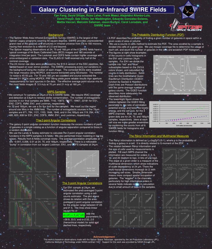
1. Galaxy Clustering in Far-Infrared SWIRE Fields Fan Fang, David Shupe, Russ Laher, Frank Masci, Alejandro Afonso-Luis, David Frayer, Seb Oliver, Ian Waddington, Eduardo Gonzalez-Solares, Mattia Vaccari, Malcolm Salaman, Jason Surace, Carol Lonsdale, and SWIRE team The Probability Distribution Function (PDF) • Background • The Spitzer Wide-Area Infrared Extragalactic Survey (SWIRE) is the largest of the Spitzer Legacy programs covering 50 square degrees. SWIRE provides unprecedented grand view of the galaxies and structures in infrared universe from 3.6 to 160 microns, tracing their evolution to a redshift of 2.5 and beyond. • The Spitzer mapping observations at 24, 70 and 160 µm of the 6 SWIRE fields have a typical coverage of 44 Basic Calibrated Data (BCD) images and 160 seconds of integration time per point. The Lockman and CDFS fields contain higher coverage with once-embargoed or validation data. The ELAIS-S1 field received only half of the nominal coverage. • The 24 micron raw data were processed by the S10.5 version of the SSC pipelines, flat-fielded based on scan mirror position.  The SWIRE processing evens out variations in the background using the median of each image. The corrected BCDs were coadded into large mosaics using MOPEX, and source extracted using SExtractor.  The nominal 1σ noise is 45-50 µJy. For 70 and 160 µm we coadded and source extracted the filtered S11 BCDs using MOPEX. PRF fitting yields more reliable results than aperture measurements for faint sources in Ge data.  The effective average point-source rms for the most fields images is  3.5 mJy at 70 µm and 21 mJy at 160 µm. • A PDF describes the probability of finding a given number of galaxies in space within a given scale of area or volume. • We use a counts-in-cells method to estimate the PDF. The area covered by a sample is divided into cells of a given size. We use mosaic coverage file to determine the usage of each cell, and count the number of galaxies in the cells and establish PDF histogram. • The figures at right show examples of the counts-in-cells histograms in the EN1 and Lockman 24μm samples. For EN1 we divide the sample into “red” and “blue” subsamples based on the 24/3.6 colors shown, and calculated the counts-in-cells distribution. Solid-lines are the Gravitational Quasi-Equilibrium Distribution (GQED) function by Saslaw & Hamilton. Dash-lines are Poisson distributions with the same average number of galaxy counts. The GQED function describes more adequately the observed distribution. • The lower-right figure shows the relation between the GQED fitting parameter b, the ratio of correlation potential energy and twice the kinetic energy, and the cell size, for the 3 MIPS channels. Blue, red, and green dots are for 24, 70, and 160μm samples, respectively. Here at each cell size we make greater ensembles by combining the counts from all 6 SWIRE fields for histograms and function fitting. • MIPS Samples • We construct 7σ samples at 24µm in the 6 SWIRE fields. We require IRAC coverage and detection at 3.6µm to remove stellar contamination. The number of extragalactic sources in our final samples are 6895, 7142, 15872, 18677, 19907, 22181 for ES1, EN2, CDFS, XMM, EN1, and Lockman, respectively. • In 70 and 160µm, we use a 5σ flux limit for the samples. We mask out the region around star Mira in the XMM field. The number of extragalactic sources in the 70µm samples are 671, 784, 1121, 1103, 1646, 1646, and in the 160µm are 119, 294, 416, 480, 620, 608 for ES1, EN2, CDFS, XMM, EN1, and Lockman, respectively. The 2-point Angular Correlations • The galaxy 2-point angular correlation function measures the excess numbers of pairs of galaxies in a single catalog as a function of angular separation compared to those in a random distribution. • We use the Landy & Szalay estimator to calculate the 2-point angular correlation functions in the MIPS samples in 6 fields. We also performed linear modeling in log-log space. Results from 6 fields converge nicely. The average correlation amplitudes at 1° are ~0.001, 0.006, 0.01 at 24, 70, and 160µm, respectively. There is a noticeable “bump” in correlation from our largest Lockman, EN1, and CDFS samples at 24µm. The Rényi Information and Multifractal Measures • The Rényi information is defined as Iß=(logΣpß)/(ß-1), where p is the probability of finding a galaxy in a cell. It is directly related to ß-moment of the PDF. • The relation between Rényi information and the size of cells used for measurements is plotted. For each MIPS channel the information are measured for orders 2, 3, 5, 10, and 20 (bottom to top), in bits of unit log2. • The slope at a given order is a measure of the multifractal dimension, which show indications of scale-dependency at 24 µm. There the multi-fractal dimensions increase (to 2) with increasing cell-sizes. Smaller dimension means more compact spatial occupation of galaxies. The “wiggles” in Ge channels, particularly for high information orders in several fields indicate noises in calculation due to small amount of data in the samples. The 3-point Angular Correlations • For EN1 sample at 24µm, we estimated the area-averaged 3-point angular correlation using a cell-counts estimator. The plot above shows its relation with the area-averaged 2-point angular correlation for the angular range between 0°.05 and 0°.5. The lines show linear square fits of • with the • parameters S3 =39.9, 33.5, and α=2.52, 2.0 (hierarchical model) for solid and dashed lines, respectively. Acknowledgement This work is based on observations made with the Spitzer Space Telescope, operated by the Jet Propulsion Laboratory (JPL), California Institute of Technology under NASA contract 1407. Support for this work was provided by NASA through JPL.