Theorems about mean, variance

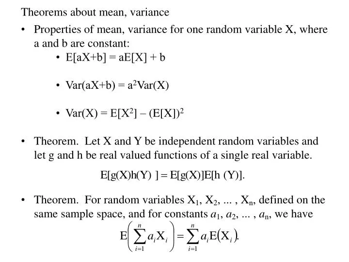
1. Theorems about mean, variance • Properties of mean, variance for one random variable X, where a and b are constant: • E[aX+b] = aE[X] + b • Var(aX+b) = a2Var(X) • Var(X) = E[X2] – (E[X])2 • Theorem. Let X and Y be independent random variables and let g and h be real valued functions of a single real variable. • Theorem. For random variables X1, X2, ... , Xn, defined on the same sample space, and for constants a1, a2, ... , an, we have

2. Mean and median may differ • Consider an exponential r. v. with λ = 1. The density is: • Note that the mean µ and the median m are different. The density has a lot of weight “in the tail” which causes the mean to be larger. We say that this density is “skewed to the right”. m = 0.693 µ=1

3. Statistical Estimation • Suppose we are given a random variable X with some unknown probability distribution. We want to estimate the basic parameters of this distribution, like the expectation of X and the variance of X. • The usual way to do this is to observe n independent variables all with the same distribution as X. To estimate the unknown mean  of X, we use the sample mean described on the next slide. The value of the observations yield a value for the sample mean which is used as an estimate for . In a similar way, the sample variance (discussed later) is used to estimate the variance of X.

4. The sample mean • Let X1,X2,…,Xn be independent and identically distributed random variables having c. d. f. F and expected value μ. Such a sequence of random variables is said to constitute a sample from the distribution F. The sample mean is denoted by and is defined by • By using the theorem on the previous slide, we have • Thus, the expected value of the sample mean is μ, the mean of the distribution. For this reason, is said to be an unbiased estimator of μ. • The random variable is an example of a statistic. That is, it is a function of the observations which does not depend on the unknown parameter μ.

5. Expectation of Bernoulli and binomial random variables • Recall that a Bernoulli random variable Xi is defined by • Since Xi is a discrete random variable, we have • Let X be a binomial random variable with parameters (n, p). Then X = X1+ X2+…+ Xn where each Xi is Bernoulli. By the theorem from the previous slide, which agrees with the direct computation we did earlier.

6. Covariance, variance of sums, and correlation Definition. The covariance between r.v.’s X and Y, denoted by Cov(X,Y), is defined by • Theorem. • Corollary. If X and Y are independent, then Cov(X, Y) = 0. • Example. Two dependent r. v.'s X and Y might have Cov(X, Y) = 0. Let X be uniform over (–1, 1) and let Y = X2.

7. Properties of covariance • Let X and Y be random variables. Then • If we take Yj = Xj, then (iv) implies that • If Xi and Xj are independent when i and j differ, then the latter equation becomes

8. Sample variance • Let X1,X2,…,Xn be independent and identically distributed random variables having c. d. f. F, expected value μ, and variance 2. Let be the sample mean. The random variable is called the sample variance. • Using the results from previous slides, we have

9. Variance of a binomial random variable • Recall that a Bernoulli random variable Xi is defined by Also, Var(Xi) = p – p2 as an easy computation shows (taking advantage of the fact that • Let X be a binomial random variable with parameters (n, p). Then X = X1+ X2+…+ Xn where each Xi is Bernoulli. By the result from a previous slide, • Upon combining the above results, we have which agrees with our earlier result.

10. Possible relations between two random variables, X and Y • For random variables X and Y, Cov(X,Y) might be positive, negative, or zero. • If Cov(X, Y) > 0, then X and Y decrease together or increase together. In this case, we say X and Y are positively correlated. • If Cov(X, Y) < 0, then X increase while Y decreases or vice versa. In this case, we say X and Y are negatively correlated. • If Cov(X, Y) = 0, we say that X and Y are uncorrelated. Recall that uncorrelated random variables may be dependent, however.