Download
1 / 98
980 likes | 1.01k Vues
This review covers first-order logic and its application in knowledge representation. Topics include syntax, semantics, terms, atomic sentences, connectives, variables, and logical quantifiers.

E N D
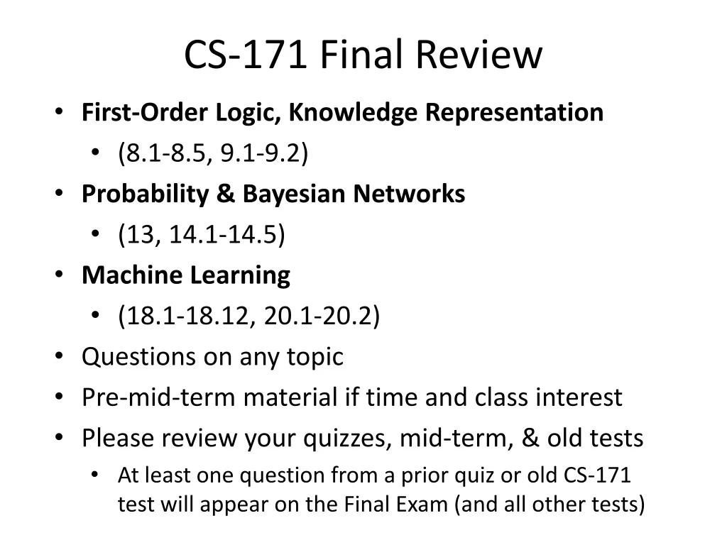
CS-171 Final Review • First-Order Logic, Knowledge Representation • (8.1-8.5, 9.1-9.2) • Probability & Bayesian Networks • (13, 14.1-14.5) • Machine Learning • (18.1-18.12, 20.1-20.2) • Questions on any topic • Pre-mid-term material if time and class interest • Please review your quizzes, mid-term, & old tests • At least one question from a prior quiz or old CS-171 test will appear on the Final Exam (and all other tests)
Knowledge Representation using First-Order Logic • Propositional Logic is Useful --- but has Limited Expressive Power • First Order Predicate Calculus (FOPC), or First Order Logic (FOL). • FOPC has greatly expanded expressive power, though still limited. • New Ontology • The world consists of OBJECTS (for propositional logic, the world was facts). • OBJECTS have PROPERTIES and engage in RELATIONS and FUNCTIONS. • New Syntax • Constants, Predicates, Functions, Properties, Quantifiers. • New Semantics • Meaning of new syntax. • Knowledge engineering in FOL
Review: Syntax of FOL: Basic elements • Constants KingJohn, 2, UCI,... • Predicates Brother, >,... • Functions Sqrt, LeftLegOf,... • Variables x, y, a, b,... • Connectives , , , , • Equality = • Quantifiers ,
Syntax of FOL: Basic syntax elements are symbols • Constant Symbols: • Stand for objects in the world. • E.g., KingJohn, 2, UCI, ... • Predicate Symbols • Stand for relations (maps a tuple of objects to a truth-value) • E.g., Brother(Richard, John), greater_than(3,2), ... • P(x, y) is usually read as “x is P of y.” • E.g., Mother(Ann, Sue) is usually “Ann is Mother of Sue.” • Function Symbols • Stand for functions (maps a tuple of objects to an object) • E.g., Sqrt(3), LeftLegOf(John), ... • Model (world)= set of domain objects, relations, functions • Interpretation maps symbols onto the model (world) • Very many interpretations are possible for each KB and world! • Job of the KB is to rule out models inconsistent with our knowledge.
Syntax of FOL: Terms • Term = logical expression that refers to an object • There are two kinds of terms: • Constant Symbols stand for (or name) objects: • E.g., KingJohn, 2, UCI, Wumpus, ... • Function Symbols map tuples of objects to an object: • E.g., LeftLeg(KingJohn), Mother(Mary), Sqrt(x) • This is nothing but a complicated kind of name • No “subroutine” call, no “return value”
Syntax of FOL: Atomic Sentences • Atomic Sentences state facts (logical truth values). • An atomic sentence is a Predicate symbol, optionally followed by a parenthesized list of any argument terms • E.g., Married( Father(Richard), Mother(John) ) • An atomic sentence asserts that some relationship (some predicate) holds among the objects that are its arguments. • An Atomic Sentence is true in a given model if the relation referred to by the predicate symbol holds among the objects (terms) referred to by the arguments.
Syntax of FOL: Connectives & Complex Sentences • Complex Sentences are formed in the same way, and are formed using the same logical connectives, as we already know from propositional logic • The Logical Connectives: • biconditional • implication • and • or • negation • Semantics for these logical connectives are the same as we already know from propositional logic.
Syntax of FOL: Variables • Variables range over objects in the world. • A variable is like a term because it represents an object. • A variable may be used wherever a term may be used. • Variables may be arguments to functions and predicates. • (A term with NO variables is called a ground term.) • (A variable not bound by a quantifier is called free.)
Syntax of FOL: Logical Quantifiers • There are two Logical Quantifiers: • Universal: x P(x) means “For all x, P(x).” • The “upside-down A” reminds you of “ALL.” • Existential: x P(x) means “There exists x such that, P(x).” • The “upside-down E” reminds you of “EXISTS.” • Syntactic “sugar” --- we really only need one quantifier. • x P(x) x P(x) • x P(x) x P(x) • You can ALWAYS convert one quantifier to the other. • RULES: and • RULE: To move negation “in” across a quantifier, change the quantifier to “the other quantifier” and negate the predicate on “the other side.” • x P(x) x P(x) • x P(x) x P(x)
Universal Quantification • means “for all” • Allows us to make statements about all objects that have certain properties • Can now state general rules: x King(x) => Person(x) “All kings are persons.” x Person(x) => HasHead(x) “Every person has a head.” • i Integer(i) => Integer(plus(i,1)) “If i is an integer then i+1 is an integer.” Note that • x King(x) Person(x) is not correct! This would imply that all objects x are Kings and are People • x King(x) => Person(x) is the correct way to say this Note that => is the natural connective to use with .
Existential Quantification • x means “there exists an x such that….” (at least one object x) • Allows us to make statements about some object without naming it • Examples: x King(x) “Some object is a king.” x Lives_in(John, Castle(x)) “John lives in somebody’s castle.” iInteger(i) GreaterThan(i,0) “Some integer is greater than zero.” Note that is the natural connective to use with (And remember that => is the natural connective to use with )
Combining Quantifiers --- Order (Scope) The order of “unlike” quantifiers is important. x y Loves(x,y) • For everyone (“all x”) there is someone (“exists y”) whom they love • y x Loves(x,y) - there is someone (“exists y”) whom everyone loves (“all x”) Clearer with parentheses: y ( x Loves(x,y) ) The order of “like” quantifiers does not matter. x y P(x, y) y x P(x, y) x y P(x, y) y x P(x, y)
De Morgan’s Law for Quantifiers Generalized De Morgan’s Rule De Morgan’s Rule Rule is simple: if you bring a negation inside a disjunction or a conjunction, always switch between them (or and, and or).
More fun with sentences • “All persons are mortal.” • [Use: Person(x), Mortal (x) ] • ∀x Person(x) Mortal(x) • ∀x ¬Person(x) ˅ Mortal(x) • Common Mistakes: • ∀x Person(x) Mortal(x) • Note that => is the natural connective to use with .
More fun with sentences • “Fifi has a sister who is a cat.” • [Use: Sister(Fifi, x), Cat(x) ] • ∃x Sister(Fifi, x) Cat(x) • Common Mistakes: • ∃x Sister(Fifi, x) Cat(x) • Note that is the natural connective to use with
More fun with sentences • “For every food, there is a person who eats that food.” • [Use: Food(x), Person(y), Eats(y, x) ] • All are correct: • ∀x ∃y Food(x) [ Person(y) Eats(y, x) ] • ∀x Food(x) ∃y [ Person(y) Eats(y, x) ] • ∀x ∃y ¬Food(x) ˅ [ Person(y) Eats(y, x) ] • ∀x ∃y [ ¬Food(x) ˅ Person(y) ] [¬ Food(x) ˅ Eats(y, x) ] • ∀x ∃y [ Food(x) Person(y) ] [ Food(x) Eats(y, x) ] • Common Mistakes: • ∀x ∃y [ Food(x) Person(y) ] Eats(y, x) • ∀x ∃y Food(x) Person(y) Eats(y, x)
More fun with sentences • “Every person eats every food.” • [Use: Person (x), Food (y), Eats(x, y) ] • ∀x ∀y [ Person(x) Food(y) ] Eats(x, y) • ∀x ∀y ¬Person(x) ˅ ¬Food(y) ˅ Eats(x, y) • ∀x ∀y Person(x) [ Food(y) Eats(x, y) ] • ∀x ∀y Person(x) [ ¬Food(y) ˅ Eats(x, y) ] • ∀x ∀y ¬Person(x) ˅ [ Food(y) Eats(x, y) ] • Common Mistakes: • ∀x ∀y Person(x) [Food(y) Eats(x, y) ] • ∀x ∀y Person(x) Food(y) Eats(x, y)
More fun with sentences • “All greedy kings are evil.” • [Use: King(x), Greedy(x), Evil(x) ] • ∀x [ Greedy(x) King(x) ] Evil(x) • ∀x ¬Greedy(x) ˅ ¬King(x) ˅ Evil(x) • ∀x Greedy(x) [ King(x) Evil(x) ] • Common Mistakes: • ∀x Greedy(x) King(x) Evil(x)
More fun with sentences • “Everyone has a favorite food.” • [Use: Person(x), Food(y), Favorite(y, x) ] • ∀x ∃y Person(x) [ Food(y) Favorite(y, x) ] • ∀x Person(x) ∃y [ Food(y) Favorite(y, x) ] • ∀x ∃y ¬Person(x) ˅ [ Food(y) Favorite(y, x) ] • ∀x ∃y [ ¬Person(x) ˅ Food(y) ] [ ¬Person(x) ˅ Favorite(y, x) ] • ∀x ∃y [Person(x) Food(y) ] [ Person(x) Favorite(y, x) ] • Common Mistakes: • ∀x ∃y [ Person(x) Food(y) ] Favorite(y, x) • ∀x ∃y Person(x) Food(y) Favorite(y, x)
Semantics: Interpretation • An interpretation of a sentence (wff) is an assignment that maps • Object constant symbols to objects in the world, • n-ary function symbols to n-ary functions in the world, • n-ary relation symbols to n-ary relations in the world • Given an interpretation, an atomic sentence has the value “true” if it denotes a relation that holds for those individuals denoted in the terms. Otherwise it has the value “false.” • Example: Kinship world: • Symbols = Ann, Bill, Sue, Married, Parent, Child, Sibling, … • World consists of individuals in relations: • Married(Ann,Bill) is false, Parent(Bill,Sue) is true, … • Your job, as a Knowledge Engineer, is to construct KB so it is true *exactly* for your world and intended interpretation.
Semantics: Models and Definitions • An interpretation and possible world satisfies a wff (sentence) if the wff has the value “true” under that interpretation in that possible world. • A domain and an interpretation that satisfies a wff is a model of that wff • Any wff that has the value “true” in all possible worlds and under all interpretations is valid. • Any wff that does not have a model under any interpretation is inconsistent or unsatisfiable. • Any wff that is true in at least one possible world under at least one interpretation is satisfiable. • If a wff w has a value true under all the models of a set of sentences KB then KB logically entails w.
Unification • Recall: Subst(θ, p) = result of substituting θ into sentence p • Unify algorithm: takes 2 sentences p and q and returns a unifier if one exists Unify(p,q) = θ where Subst(θ, p) = Subst(θ, q) • Example: p = Knows(John,x) q = Knows(John, Jane) Unify(p,q) = {x/Jane}
Unification examples • simple example: query = Knows(John,x), i.e., who does John know? p q θ Knows(John,x) Knows(John,Jane) {x/Jane} Knows(John,x) Knows(y,OJ) {x/OJ,y/John} Knows(John,x) Knows(y,Mother(y)) {y/John,x/Mother(John)} Knows(John,x) Knows(x,OJ) {fail} • Last unification fails: only because x can’t take values John and OJ at the same time • But we know that if John knows x, and everyone (x) knows OJ, we should be able to infer that John knows OJ • Problem is due to use of same variable x in both sentences • Simple solution: Standardizing apart eliminates overlap of variables, e.g., Knows(z,OJ)
Unification • To unify Knows(John,x) and Knows(y,z), θ = {y/John, x/z } or θ = {y/John, x/John, z/John} • The first unifier is more general than the second. • There is a single most general unifier (MGU) that is unique up to renaming of variables. MGU = { y/John, x/z } • General algorithm in Figure 9.1 in the text
Knowledge engineering in FOL • Identify the task • Assemble the relevant knowledge • Decide on a vocabulary of predicates, functions, and constants • Encode general knowledge about the domain • Encode a description of the specific problem instance • Pose queries to the inference procedure and get answers • Debug the knowledge base
The electronic circuits domain • Identify the task • Does the circuit actually add properly? • Assemble the relevant knowledge • Composed of wires and gates; Types of gates (AND, OR, XOR, NOT) • Irrelevant: size, shape, color, cost of gates • Decide on a vocabulary • Alternatives: Type(X1) = XOR (function) Type(X1, XOR) (binary predicate) XOR(X1) (unary predicate)
The electronic circuits domain • Encode general knowledge of the domain • t1,t2 Connected(t1, t2) Signal(t1) = Signal(t2) • t Signal(t) = 1 Signal(t) = 0 • 1 ≠ 0 • t1,t2 Connected(t1, t2) Connected(t2, t1) • g Type(g) = OR Signal(Out(1,g)) = 1 n Signal(In(n,g)) = 1 • g Type(g) = AND Signal(Out(1,g)) = 0 n Signal(In(n,g)) = 0 • g Type(g) = XOR Signal(Out(1,g)) = 1 Signal(In(1,g)) ≠ Signal(In(2,g)) • g Type(g) = NOT Signal(Out(1,g)) ≠ Signal(In(1,g))
The electronic circuits domain • Encode the specific problem instance Type(X1) = XOR Type(X2) = XOR Type(A1) = AND Type(A2) = AND Type(O1) = OR Connected(Out(1,X1),In(1,X2)) Connected(In(1,C1),In(1,X1)) Connected(Out(1,X1),In(2,A2)) Connected(In(1,C1),In(1,A1)) Connected(Out(1,A2),In(1,O1)) Connected(In(2,C1),In(2,X1)) Connected(Out(1,A1),In(2,O1)) Connected(In(2,C1),In(2,A1)) Connected(Out(1,X2),Out(1,C1)) Connected(In(3,C1),In(2,X2)) Connected(Out(1,O1),Out(2,C1)) Connected(In(3,C1),In(1,A2))
The electronic circuits domain • Pose queries to the inference procedure What are the possible sets of values of all the terminals for the adder circuit? i1,i2,i3,o1,o2 Signal(In(1,C1)) = i1 Signal(In(2,C1)) = i2 Signal(In(3,C1)) = i3 Signal(Out(1,C1)) = o1 Signal(Out(2,C1)) = o2 • Debug the knowledge base May have omitted assertions like 1 ≠ 0
CS-171 Final Review • First-Order Logic, Knowledge Representation • (8.1-8.5, 9.1-9.2) • Probability & Bayesian Networks • (13, 14.1-14.5) • Machine Learning • (18.1-18.12, 20.1-20.2) • Questions on any topic • Pre-mid-term material if time and class interest • Please review your quizzes, mid-term, & old tests • At least one question from a prior quiz or old CS-171 test will appear on the Final Exam (and all other tests)
CS-171 Final Review • First-Order Logic, Knowledge Representation • (8.1-8.5, 9.1-9.2) • Probability & Bayesian Networks • (13, 14.1-14.5) • Machine Learning • (18.1-18.12, 20.1-20.2) • Questions on any topic • Pre-mid-term material if time and class interest • Please review your quizzes, mid-term, & old tests • At least one question from a prior quiz or old CS-171 test will appear on the Final Exam (and all other tests)
You will be expected to know • Basic probability notation/definitions: • Probability model, unconditional/prior and conditional/posterior probabilities, factored representation (= variable/value pairs), random variable, (joint) probability distribution, probability density function (pdf), marginal probability, (conditional) independence, normalization, etc. • Basic probability formulae: • Probability axioms, product rule, Bayes’ rule. • How to use Bayes’ rule: • Naïve Bayes model (naïve Bayes classifier)
Probability • P(a) is the probability of proposition “a” • e.g., P(it will rain in London tomorrow) • The proposition a is actually true or false in the real-world • Probability Axioms: • 0 ≤ P(a) ≤ 1 • P(NOT(a)) = 1 – P(a) => SA P(A) = 1 • P(true) = 1 • P(false) = 0 • P(A OR B) = P(A) + P(B) – P(A AND B) • Any agent that holds degrees of beliefs that contradict these axioms will act irrationally in some cases • Rational agents cannot violate probability theory. • Acting otherwise results in irrational behavior.
Concepts of Probability • Unconditional Probability • P(a),the probability of “a” being true, or P(a=True) • Does not depend on anything else to be true (unconditional) • Represents the probability prior to further information that may adjust it (prior) • Conditional Probability • P(a|b),the probability of “a” being true, given that “b” is true • Relies on “b” = true (conditional) • Represents the prior probability adjusted based upon new information “b” (posterior) • Can be generalized to more than 2 random variables: • e.g. P(a|b, c, d) • Joint Probability • P(a, b) = P(a ˄ b),the probability of “a” and “b” both being true • Can be generalized to more than 2 random variables: • e.g. P(a, b, c, d)
Random Variables • Random Variable: • Basic element of probability assertions • Similar to CSP variable, but values reflect probabilities not constraints. • Variable: A • Domain: {a1, a2, a3} <-- events / outcomes • Types of Random Variables: • Boolean random variables = { true, false } • e.g., Cavity (= do I have a cavity?) • Discrete random variables = One value from a set of values • e.g., Weather is one of <sunny, rainy, cloudy ,snow> • Continuous random variables = A value from within constraints • e.g., Current temperature is bounded by (10°, 200°) • Domain values must be exhaustive and mutually exclusive: • One of the values must always be the case (Exhaustive) • Two of the values cannot both be the case (Mutually Exclusive)
Basic Probability Relationships • P(A) + P( A) = 1 • Implies that P(A) = 1 ─ P(A) • P(A, B) = P(A ˄ B) = P(A) + P(B) ─ P(A ˅ B) • Implies that P(A ˅ B) = P(A) + P(B) ─ P(A ˄ B) • P(A | B) = P(A, B) / P(B) • Conditional probability; “Probability of A given B” • P(A, B) = P(A | B) P(B) • Product Rule (Factoring); applies to any number of variables • P(a, b, c,…z) = P(a | b, c,…z) P(b | c,...z) P(c|...z)...P(z) • P(A) = B,C P(A, B, C) • Sum Rule (Marginal Probabilities); for any number of variables • P(A, D) = BC P(A, B, C, D) • P(B | A) = P(A | B) P(B) / P(A) • Bayes’ Rule; for any number of variables You need to know these !
Summary of Probability Rules • Product Rule: • P(a, b) = P(a|b) P(b) = P(b|a) P(a) • Probability of “a” and “b” occurring is the same as probability of “a” occurring given “b” is true, times the probability of “b” occurring. • e.g., P( rain, cloudy ) = P(rain | cloudy) * P(cloudy) • Sum Rule: (AKA Law of Total Probability) • P(a) = Sb P(a, b) = Sb P(a|b) P(b), where B is any random variable • Probability of “a” occurring is the same as the sum of all joint probabilities including the event, provided the joint probabilities represent all possible events. • Can be used to “marginalize” out other variables from probabilities, resulting in prior probabilities also being called marginal probabilities. • e.g., P(rain) = SWindspeed P(rain, Windspeed) where Windspeed = {0-10mph, 10-20mph, 20-30mph, etc.} • Bayes’ Rule: • P(b|a) = P(a|b) P(b) / P(a) • Acquired from rearranging the product rule. • Allows conversion between conditionals, from P(a|b) to P(b|a). • e.g., b = disease, a = symptoms More natural to encode knowledge as P(a|b) than as P(b|a).
Full Joint Distribution • We can fully specify a probability space by constructing a full joint distribution: • A full joint distribution contains a probability for every possible combination of variable values. • E.g., P( J=f M=t A=t B=t E=f ) • From a full joint distribution, the product rule, sum rule, and Bayes’ rule can create any desired joint and conditional probabilities.
Independence • Formal Definition: • 2 random variables A and B are independent iff: P(a, b) = P(a) P(b), for all values a, b • Informal Definition: • 2 random variables A and B are independent iff: P(a | b) = P(a) OR P(b | a) = P(b), for all values a, b • P(a | b) = P(a) tells us that knowing b provides no change in our probability for a, and thus b contains no information about a. • Also known as marginal independence, as all other variables have been marginalized out. • In practice true independence is very rare: • “butterfly in China” effect • Conditional independence is much more common and useful
Conditional Independence • Formal Definition: • 2 random variables A and B are conditionally independent given C iff: P(a, b|c) = P(a|c) P(b|c), for all values a, b, c • Informal Definition: • 2 random variables A and B are conditionally independent given C iff: P(a|b, c) = P(a|c) OR P(b|a, c) = P(b|c), for all values a, b, c • P(a|b, c) = P(a|c) tells us that learning about b, given that we already know c, provides no change in our probability for a, and thus b contains no information about a beyond what c provides. • Naïve Bayes Model: • Often a single variable can directly influence a number of other variables, all of which are conditionally independent, given the single variable. • E.g., k different symptom variables X1, X2, … Xk, and C = disease, reducing to: P(X1, X2,…. XK | C) = P P(Xi | C)
Examples of Conditional Independence • H=Heat, S=Smoke, F=Fire • P(H, S | F) = P(H | F) P(S | F) • P(S | F, S) = P(S | F) • If we know there is/is not a fire, observing heat tells us no more information about smoke • F=Fever, R=RedSpots, M=Measles • P(F, R | M) = P(F | M) P(R | M) • P(R | M, F) = P(R | M) • If we know we do/don’t have measles, observing fever tells us no more information about red spots • C=SharpClaws, F=SharpFangs, S=Species • P(C, F | S) = P(C | S) P(F | S) • P(F | S, C) = P(F | S) • If we know the species, observing sharp claws tells us no more information about sharp fangs
Review Bayesian Networks (Chapter 14.1-5) • You will be expected to know: • Basic concepts and vocabulary of Bayesian networks. • Nodes represent random variables. • Directed arcs represent (informally) direct influences. • Conditional probability tables, P( Xi | Parents(Xi) ). • Given a Bayesian network: • Write down the full joint distribution it represents. • Inference by Variable Elimination • Given a full joint distribution in factored form: • Draw the Bayesian network that represents it. • Given a variable ordering and background assertions of conditional independence among the variables: • Write down the factored form of the full joint distribution, as simplified by the conditional independence assertions.
The full joint distribution The graph-structured approximation Bayesian Networks • Represent dependence/independence via a directed graph • Nodes = random variables • Edges = direct dependence • Structure of the graph Conditional independence • Recall the chain rule of repeated conditioning: • Requires that graph is acyclic (no directed cycles) • 2 components to a Bayesian network • The graph structure (conditional independence assumptions) • The numerical probabilities (of each variable given its parents)
B A C Bayesian Network • A Bayesian network specifies a joint distribution in a structured form: • Dependence/independence represented via a directed graph: • Node = random variable • Directed Edge = conditional dependence • Absence of Edge = conditional independence • Allows concise view of joint distribution relationships: • Graph nodes and edges show conditional relationships between variables. • Tables provide probability data. Full factorization p(A,B,C) = p(C|A,B)p(A|B)p(B) = p(C|A,B)p(A)p(B) After applying conditional independence from the graph
A B C Examples of 3-way Bayesian Networks Independent Causes: p(A,B,C) = p(C|A,B)p(A)p(B) “Explaining away” effect: Given C, observing A makes B less likely e.g., earthquake/burglary/alarm example A and B are (marginally) independent but become dependent once C is known You heard alarm, and observe Earthquake …. It explains away burglary Independent Causes A Earthquake B Burglary C Alarm Nodes: Random Variables A, B, C Edges: P(Xi | Parents) Directed edge from parent nodes to Xi A C B C
A B C Examples of 3-way Bayesian Networks Marginal Independence: p(A,B,C) = p(A) p(B) p(C) Nodes: Random Variables A, B, C Edges: P(Xi | Parents) Directed edge from parent nodes to Xi No Edge!
A C B Extended example of 3-way Bayesian Networks Common Cause A : Fire B: Heat C: Smoke Conditionally independent effects: p(A,B,C) = p(B|A)p(C|A)p(A) B and C are conditionally independent Given A “Where there’s Smoke, there’s Fire.” If we see Smoke, we can infer Fire. If we see Smoke, observing Heat tells us very little additional information.
A B C Examples of 3-way Bayesian Networks Markov dependence: p(A,B,C) = p(C|B) p(B|A)p(A) A affects B and B affects C Given B, A and C are independent e.g. If it rains today, it will rain tomorrow with 90% On Wed morning… If you know it rained yesterday, it doesn’t matter whether it rained on Mon Markov Dependence A Rain on Mon B Ran on Tue C Rain on Wed Nodes: Random Variables A, B, C Edges: P(Xi | Parents) Directed edge from parent nodes to Xi A B B C