Download
1 / 15
150 likes | 273 Vues
Physics 434 Module 3. Acoustic excitation of a physical system. The theme of the next three weeks. Physical system (the tube). Output signal. Input signal. This week: operate in the frequency domain For a given frequency, what is the response? (resonances, etc.) Next week: time domain

E N D
Physics 434 Module 3 Acoustic excitation of a physical system Physics 434 Module 3 - T. Burnett
The theme of the next three weeks Physical system(the tube) Output signal Input signal • This week: operate in the frequency domain • For a given frequency, what is the response? (resonances, etc.) • Next week: time domain • Excite with a pulse, measure response • Following week: Fourier transform • Relate to frequency domain measurement
Goals for this module • Control and monitor an applied frequency • Detect and measure a sound wave • Generate set of RMS values vs. frequency • Fit resonances to determine resonant frequencies and “Q” values • Check speed of sound from resonance difference Physics 434 Module 3 - T. Burnett
Kundt’s tube • Read the Wikipedia article for the history • From 1866: glass tube, used to measure speed of sound • Like an organ pipe. • End effects make simple frequency vs. length not like a stretched string Physics 434 Module 3 - T. Burnett
Step 1– just electronics ‘scope: tube speaker from microphone Physics 434 Module 3 - T. Burnett
Step 1, cont • Wiring summary for the preamp box: • Microphone→ MIC IN • MIC OUT → scope ch 2 → ach0 • dac0 → scope ch 1 → SPEAKER IN • SPEAKER OUT → speaker • Using signal generator, adjust amplifier gains for given input (1 V) so that output does not saturate between 500 and 2000 Hz • Note a few resonant frequencies for later check Physics 434 Module 3 - T. Burnett
Step 2 – test the output • Get SoundGenerator.llb from module3.zip • Note that it contains several VIs: • SoundGenerator • Generate a continuous signal with selectable frequency • Generate a sequence of discrete frequencies • Measure_rms • Monitor and measure the signal acquired by the DAC • Look at the output on the scope, verify the frequency, feed it to your microphone, verify that it does not saturate. Physics 434 Module 3 - T. Burnett
The DAQ systems Physics 434 Module 3 - T. Burnett
Step 3 – check the data acquisition • The VI, measure_rms.vi, acquires a waveform, with adjustable sampling rate and sample size.. • The output is graphed and analyzed by a simple-minded RMS vi. • Check that the RMS of the signal generator output, or the output from the DAQ card is stable and does not vary with input frequency (500-2000 Hz). (We do not actually measure this, but assume that it does not change. Physics 434 Module 3 - T. Burnett
Step 4 – assemble your VI and run it • Easy to cut and paste from the two test VI’s • Must create a table of (actual) frequencies and RMS response from the microphone, with constant input to the speaker • Display on an XY graph • Write to a file with the “Write To Spreadsheet File” vi from the Programming | File I/O menu. (Or grab from demo fileio.vi in module3.zip) Set transpose to print columns Physics 434 Module 3 - T. Burnett
Read and write: see fileio.vi • Fileio.vi, in the zip. Uses write to and read from spreadsheet Physics 434 Module 3 - T. Burnett
This part sets up the demo Step 5 – Analyze the resonance peaks This is a new VI that you must write, capable of reading data from the file and fitting it: see test_resonance_fit.vi, with sub-vi resonance_fitter.vi for the fitting piece that you may use. Note: it must select a range over which the resonance is valid. The formula: Watch for this guy! Physics 434 Module 3 - T. Burnett
Submit your vi’s in an llb • Save plots with current value (can do all at once from Edit menu) • Use documentation for descriptions. • Analysis VI should have a table of the resonance parameters, and your estimate of the speed of sound Physics 434 Module 3 - T. Burnett
What it might look like Physics 434 Module 3 - T. Burnett
Summary Physics 434 Module 3 - T. Burnett Step 1: Analog exploration This is an exploratory step that does not use the computer. Instead connect the signal generator to the amplifier speaker input and the oscilloscope to the microphone output. Set the waveform to be sinusoidal, and vary the frequency from 100 to 2000 Hz, recording the approximate resonant frequencies, reading from the signal generator dial. Make a quick plot of fn vs. n, and note that the spacing is linear only above ~ 800 Hz, which differs from the naïve expectation of Eqn (1). The rest of the lab will measure these frequencies accurately. Leave the oscilloscope connected to the microphone output, to monitor the following steps. Step 2: Test the sound generator VI Set up the sound generator VI to produce a fixed frequency, 1 kHz for example. You can use a standard sweeping VI that is provided. Examine this on the oscilloscope, and verify the frequency. Step 3: Test the acquisition VI You will use a capture VI to acquire the waveform. In this step, use the analog signal generator to produce an input signal that can be acquired. A sub VI, called RMS, is provided to combine data acquisition with measurement of the RMS of a waveform. This will be your measure of the amplitude. (Look inside to understand it.) Step 4: Acquire the data As you saw in Step 1, the linear part of fn vs. n is above 800 Hz. Set the sound generator to sweep from 700 to 2000 Hz, and put your acquisition code or subVI into a loop sweeping over frequency. Acquire a table of rms amplitude vs. frequency and make a graph and write it to a file. Step 5: Fit the data This is conveniently performed off line and will demonstrate LabVIEW’s capability to perform data analysis. You want to determine the best values of the parameters fn, and Qn for several of the resonances in the linear region. (You may have to edit the file to isolate the individual resonances, or, more elegantly, have a VI select a subset.) A fitter vi has been set up for this, interfacing the resonance function to a non-linear curve fitter vi. Your output plot should show the data as open, unconnected circles and the model as a solid line, as you can see in the vi demo program. Hand in your two VI’s, from steps 4 and 5, fully commented and with documentation. The VI’s should be saved showing data and analysis results on the front panel.