Download
1 / 60
600 likes | 710 Vues
Ensemble forecasts of streamflows using large-scale climate information : applications to the trcukee-carson basin. Balaji Rajagopalan Katrina Grantz CIVIL, ENVIRONMENTAL AND ARCHITECTURAL ENGINEERING DEPARTMENT UNIVERSITY OF COLORADO AT BOULDER NCAR/ESIG Spring 2004. Inter-decadal. Climate.

E N D
Ensemble forecasts of streamflows using large-scale climate information : applications to the trcukee-carson basin Balaji Rajagopalan Katrina Grantz CIVIL, ENVIRONMENTAL AND ARCHITECTURAL ENGINEERING DEPARTMENT UNIVERSITY OF COLORADO AT BOULDER NCAR/ESIG Spring 2004
Inter-decadal Climate Decision Analysis: Risk + Values Time Horizon • Facility Planning • Reservoir, Treatment Plant Size • Policy + Regulatory Framework • Flood Frequency, Water Rights, 7Q10 flow • Operational Analysis • Reservoir Operation, Flood/Drought Preparation • Emergency Management • Flood Warning, Drought Response Data: Historical, Paleo, Scale, Models Weather Hours A Water Resources Management Perspective
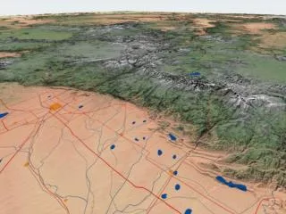
Study Area PYRAMID LAKE WINNEMUCCA LAKE (dry) CALIFORNIA NEVADA Nixon Stillwater NWR Derby Dam STAMPEDE Reno/Sparks Fernley Fallon TRUCKEE RIVER INDEPENDENCE BOCA Newlands Project PROSSER Truckee CARSON LAKE MARTIS LAHONTAN Carson City DONNER Tahoe City CARSON RIVER LAKE TAHOE NEVADA Truckee Carson CALIFORNIA TRUCKEE CANAL Farad Ft Churchill
Study Area Lahontan Reservoir Prosser Creek Dam
Motivation • USBR needs good seasonal forecasts on Truckee and Carson Rivers • Forecasts determine how storage targets will be met on Lahonton Reservoir to supply Newlands Project Truckee Canal
Basin Precipitation NEVADA Truckee Carson CALIFORNIA Average Annual Precipitation
Data Used • 1949-2003 monthly data sets: • Natural Streamflow (Farad & Ft. Churchill gaging stations) (from USBR) • Snow Water Equivalent (SWE)- basin average • Large-Scale Climate Variables (SST, Winds, Z500..) from http://www.cdc.noaa.gov
Basin Climatology • Streamflow in Spring (April, May, June) • Precipitation in Winter (November – March) • Primarily snowmelt dominated basins
SWE Correlation • Winter SWE and spring runoff in Truckee and Carson Rivers are highly correlated • April 1st SWE better than March 1st SWE
Hydroclimate in Western US • Past studies have shown a link between large-scale ocean-atmosphere features (e.g. ENSO and PDO) and western US hydroclimate (precipitation and streamflow) • E.g., Pizarro and Lall (2001) Correlations between peak streamflow and Nino3
The Approach Climate Diagnostics • Climate Diagnostics To identify relevant predictors to streamflow / precipitation • Forecasting Model stochastic models for ensemble forecasting - conditioned on climate information Forecasting Model Decision Support System • Decision Support System (DSS) Couple forecast with DSS to demonstrate utility of forecast
Correlations between spring flows and winter (standard) climate indices (NINO3, PNA, PDO etc.) were close to 0! • Need to explore other regions correlation maps of ocean-atmospheric variables?
Winter Climate Correlations Truckee Spring Flow 500mb Geopotential Height Sea Surface Temperature
Fall Climate Correlations Carson Spring Flow Sea Surface Temperature 500 mb Geopotential Height
Climate Indices • Use areas of highest correlation to develop indices to be used as predictors in the forecasting model • Area averages of geopotential height and SST 500 mb Geopotential Height Sea Surface Temperature
Forecasting Model Predictors • SWE • Geopotential Height • Sea Surface Temperature
Persistence of Climate Patterns Strongest correlation in Winter (Dec-Feb) Correlation statistically significant back to August
Climate Composites Vector Winds Low Streamflow Years High Streamflow Years
Climate Composites Sea Surface Temperature Low Streamflow Years High Streamflow Years
Physical Mechanism • Winds rotate counter-clockwise around area of low pressure bringing warm, moist air to mountains in Western US L
Climate Diagnostics Summary • Winter/ Fall geopotential heights and SSTs over Pacific Ocean related to Spring streamflow in Truckee and Carson Rivers • Physical explanation for this correlation • Relationships are nonlinear
Ensemble Forecast • Ensemble Forecast/Stochastic Simulation /Scenarios generation – all of them are conditional probability density function problems • Estimate conditional PDF and simulate (Monte Carlo, or Bootstrap)
Forecasting Model Requirements • Forecast spring streamflow (total volume) • Capture linear and nonlinear relationships in the data • Produce ensemble forecasts (to calculate exceedence probabilities)
Parametric Models - Drawbacks • Model selection / parameter estimation issues Select a model (PDFs or Time series models) from candidate models Estimate parameters • Limited ability to reproduce nonlinearity and non-Gaussian features. All the parametric probability distributions are ‘unimodal’ All the parametric time series models are ‘linear’
Parametric Models - Drawbacks • Models are fit on the entire data set Outliers can inordinately influence parameter estimation (e.g. a few outliers can influence the mean, variance) Mean Squared Error sense the models are optimal but locally they can be very poor. Not flexible • Not Portable across sites
Nonparametric Methods • Any functional (probabiliity density, regression etc.) estimator is nonparametric if: It is “local” – estimate at a point depends only on a few neighbors around it. (effect of outliers is removed) No prior assumption of the underlying functional form – data driven
Nonparametric Methods • Kernel Estimators (properties well studied) • Splines • Multivariate Adaptive Regression Splines (MARS) • K-Nearest Neighbor (K-NN) Bootstrap Estimators • Locally Weighted Polynomials (K-NN Polynomials)
K-NN Philosophy • Find K-nearest neighbors to the desired point x • Resample the K historical neighbors (with high probability to the nearest neighbor and low probability to the farthest) Ensembles • Weighted average of the neighbors Mean Forecast • Fit a polynomial to the neighbors – Weighted Least Squares • Use the fit to estimate the function at the desired point x (i.e. local regression) • Number of neighbors K and the order of polynomial p is obtained using GCV (Generalized Cross Validation) – K = N and p = 1 Linear modeling framework. • The residuals within the neighborhood can be resampled for providing uncertainity estimates / ensembles.
k-nearest neighborhoods A and B for xt=x*A and x*B respectively Logistic Map Example 4-state Markov Chain discretization
Modified K- Nearest Neighbor(K-NN) • Uses local polynomial for the mean forecast (nonparametric) • Bootstraps the residuals for the ensemble (stochastic) Benefits • Produces flows not seen in the historical record • Captures any non-linearities in the data, as well as linear relationships • Quantifies the uncertainty in the forecast (Gaussian and non-Gaussian)
Residual Resampling e * t y * t xt* yt* = f(xt*) + et*
Applications to date…. • Monthly Streamflow Simulation Space and time disaggregation of monthly to daily streamflow • Monte Carlo Sampling of Spatial Random Fields • Probabilistic Sampling of Soil Stratigraphy from Cores • Hurricane Track Simulation • Multivariate, Daily Weather Simulation • Downscaling of Climate Models • Ensemble Forecasting of Hydroclimatic Time Series • Biological and Economic Time Series • Exploration of Properties of Dynamical Systems • Extension to Nearest Neighbor Block Bootstrapping -Yao and Tong
Model Validation & Skill Measure • Cross-validation: drop one year from the model and forecast the “unknown” value • Compare median of forecasted vs. observed (obtain “r” value) • Rank Probability Skill Score
Model Validation & Skill Measure • Cross-validation: drop one year from the model and forecast the “unknown” value • Compare median of forecasted vs. observed (obtain “r” value) • Rank Probability Skill Score • Likelihood Skill Score (Rajagopalan et al., 2001)
Forecasting Results • Predictors • April 1st SWE • Dec-Feb geopotential height 95th 50th 5th 95th 50th 5th April 1st forecast
Forecasting Results • Ensemble forecasts provide range of possible streamflow values • Water manager can calculate exceedence probabilites Wet Year Dry Year
Forecast Skill Scores April 1st forecast • Median skill scores significantly beat climatology in all year subsets, both Truckee and Carson • Truckee slightly better than Carson
Use of Climate Index in Forecast Extremely Wet Years • In general, the boxes are much tighter with geopotential height (greater confidence) • Underprediction w/o climate index– might not be fully prepared with flood control measures 95th 95th 50th 50th 5th 5th 95th 95th 50th 50th 5th 5th SWEand Geopotential Height SWE
Use of Climate Index in Forecast Extremely Dry Years • Tighter prediction interval with geopotential height • Overprediction w/o climate index (esp. in 1992) • Might not implement necessary drought precautions in sufficient time 95th 95th 50th 50th 5th 5th 95th 95th 50th 50th 5th 5th SWEand Geopotential Height SWE
Model Skills in Water Resources Decision Support System Ensemble Forecasts are passed through a Decision Support (RIVERWARE) System of the Truckee/Carson Basin Ensembles of the decision variables are compared against the “actual” values
Truckee RiverWare Model • Physical Mechanisms • Reservoir releases, diversions, evap, reach routing • Policies • Implemented with “rules” (user defined prioritized logic) • Water Rights • Implemented in accounting network
Method to test the utility of the forecasts and the role they play in decision making Model implements major policies in lower basin (Newlands Project OCAP) Seasonal timestep Simplified Seasonal Model
Seasonal Model Policies • Use Carson water first • Max canal diversions: 164 kaf • Storage targets on Lahontan Reservoir: 2/3 of projected April-July runoff volume • Minimum Lahontan storage target: 1/3 of average historical spring runoff • No minimum fish flows
Lahontan Storage Available for Irrigation Truckee River Water Available for Fish Diversion through the Truckee Canal Decision Variables
Seasonal Model Results: 1992 • Irrigation Water less than typical– decrease crop size or use drought-resistant crops • Truckee Canal smaller diversion-start the season with small diversions (one way canal) • Very little Fish Water- releases from Stampede coordinated with Canal diversions Ensemble forecast results Climatology forecast results Observed value results NRCS official forecast results