DTFT And Fourier Transform

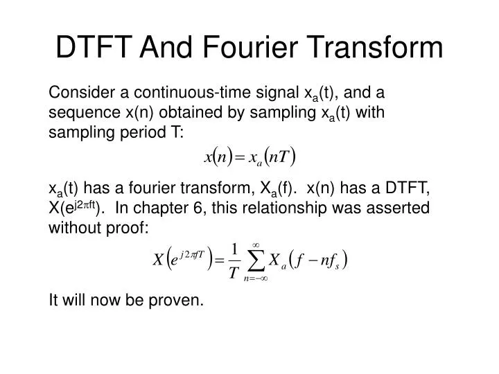
1. DTFT And Fourier Transform Consider a continuous-time signal xa(t), and a sequence x(n) obtained by sampling xa(t) with sampling period T: xa(t) has a fourier transform, Xa(f). x(n) has a DTFT, X(ej2pft). In chapter 6, this relationship was asserted without proof: It will now be proven.

2. DTFT And Fourier Transform Consider a continuous-time impluse train (Dirac impulses): s(t) -3T -2T -T 0T T 2T 3T

3. DTFT And Fourier Transform If we multiply the impulse train and xa(t), we get a weighted impulse train. The weights are the values of xa(t) at integer multiples of T. Since the product of the two signals is zero at all other times, it may also be expressed as:

4. DTFT And Fourier Transform But we’ve already seen that x(n) = xa(nT), xs(t) is a continuous time signal, which exists for all values of t, not just integer multiples of T. at t = nT, its value is that of x(n). At all other times, it is zero. We’ll now prove

5. DTFT And Fourier Transform First, we’ll show that that s(t) is periodic, with period T. It can be expressed as a Fourier series: The coefficients of the Fourier series, cn, are given by:

6. DTFT And Fourier Transform Only one of the impulses is between –T/2 and T-2, and s(t) is zero every where else between the integration limits, so: Using the sifting poperty of the continuous-time impulse,

7. DTFT And Fourier Transform So the Fourier series representation of s(t) is The Fourier transform of s(t) is

8. DTFT And Fourier Transform Since we have the following Fourier transform pair We can write the Fourier transform of s(t) as simply: Recalling that xs(t) = xa(t)s(t), we know that

9. DTFT And Fourier Transform Recalling that xs(t) = xa(t)s(t), we know that

10. DTFT And Fourier Transform And using the sifting property, The relationship we set out to prove was We’ve just shown that Xs(f) is equal to the right side of the relationship. Now we’ll show that Xs(f) is also equal to the left side, which will complete the proof.

11. DTFT And Fourier Transform Recall that So

12. DTFT And Fourier Transform Using this transform pair, We can now write: But this is the same as the DTFT of x(n), X(ejw), if w = 2pfT. Therefore, This completes the proof.

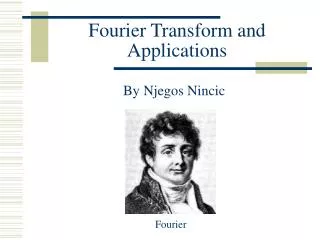
13. Xa(f) -2fs -fs -B 0 B fs 2fs f Sampling Theorem A continuous time signal xa(t) that is bandlimited to B Hz (that is, its spectrum contains no energy at any frequency above B Hz) can be completely recovered from it’s samples, xa(nT) if the sampling frequency fs (fs = 1/T) is greater than 2B. Below is a depiction of the spectrum of a bandlimited signal xa(t). A

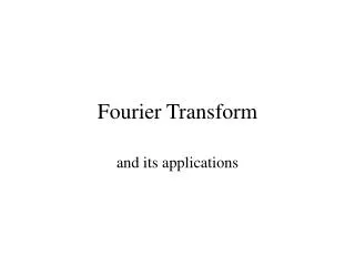
14. Sampling Theorem If fs > 2B, the sampled signal xs(t)is as depicted spectrally below: Xs(f) A/T -B B -2fs -fs 0 fs 2fs where T = 1/ fs. Spectrally, the sampled signal xs(t)is a scaled copy of xa(t) between –fs/2 and fs/2. It also contains spectral copies centered at n –fs.

15. Sampling Theorem If we use an ideal lowpass filter to strip off the unwanted spectral copies, we can perfectly recover the spectrum of the original signal xa(t) – and therefore, we also recover xa(t) itself! Again, if we have a signal xa(t) and sample it to obtain the weighted impulse train xs(t), we can recover xa(t) from xs(t) by using an ideal lowpass filter xa(t) is related to the sequence x(n) by

16. Ideal D/A Conversion If we process the sequence x(n) in a way that converts it to xs(t), then use an ideal lowpass filter to strip off the unwanted spectral copies, then we convert a digital sequence to an analo signal. This is an ideal digital to analog (D/A) converter. Convert to Impulse Train Ideal Lowpass Filter xs(t) x(n) xa(t) Gain = T Cutoff freq = fs/2

17. Ideal D/A Conversion of course, it’s impossible to make an ideal D/A converter. An ideal lowpass filter can’t be realized, and we can’t create a train of ideal impulses. Furthermore, there will always be errors due to finite word length (quantization error). There will also always be some aliasing, because no signal is perfectly bandlimited. We can approximate an impulse train, though, and we can approximate an ideal lowpass filter. Therefore, we can make an imperfect D/A converter.

18. Ideal D/A Conversion Now let’s talk about D/A conversion from a time domain viewpoint. When we filter xs(t) to remove the spectral copies and recover xa(t), we’re convolving xs(t) with the impulse response of the ideal lowpass filter.

19. Ideal D/A Conversion This process connects the “dots”, which are the magnitudes of the impulses that comprise xs(t). In otherwords, the ideal D/A conversion process is also an ideal interpolation process. Convolving the xs(t) with ha(t),

20. Ideal D/A Conversion But so,

21. Ideal D/A Conversion Rearranging, And, using the sifting property: This is the ideal interpolation formula.

22. Real-World D/A Conversion The ideal D/A converter uses the sequence x(n) to generate a weighted impulse train, xs(t). An ideal lowpass filter then “connects the dots” by smoothing the impulse train. A real D/A converter generates a series of “rectangular” pulses, weighted according to the sequence x(n).

23. xs(t) t -4T -3T -2T -T 0 T 2T 3T 4T Real-World D/A Conversion Here’s a depiction of the impulse train generated by an ideal D/A converter for some sequence x(n):

24. xp(t) t -4T -3T -2T -T 0 T 2T 3T 4T Real-World D/A Conversion Here’s the pulse train generated by a real D/A converter, overlayed with the impulse train.

25. ga(t) A t 0 T Real-World D/A Conversion The pulse train is generated by weighting a series of rectangular pulses, like the one shown here: The pulse train can be written as:

26. Real-World D/A Conversion Normally, the D/A converter does not include a lowpass filter (although the pulse train generation is a lowpass process of a sort). In most cases, a analog filter is required downstream. It we compare xp(t) to xa(t) (the original continuous-time signal), xp(t) is a staircase approximation of xa(t) .

27. Real-World D/A Conversion In the frequency domain, for the ideal converter, where Ha(f) is the transfer function of the ideal lowpass filter, and for the real converter, where Ha(f) is the Fourier transform of the rectangular pulse ga(t)

28. Real-World D/A Conversion In the frequency domain, Xp(f) is the product of Xs(f) and Ga(f). In the time domain, xp(t) is obtained by convolving xs(t) with ga(t):

29. Real-World D/A Conversion To see what this looks like spectrally, we need to know the spectrum of the retangular pulse, Ga(f). In chapter 3, we saw that the Fourier transform of the rectangular pulse shown below r(t) A t -T/2 T/2 0 was given by:

30. Real-World D/A Conversion By comparing this to ga(t), we see that ga(t) is ra(t) delayed by T/2. Therefore, by the time shifting theorem, and its amplitude response is:

31. Real-World D/A Conversion If we plot the amplitude response, it looks as shown in figure 7-8 of the textbook. Notice that, in the range of frequencies between 0 and fs/2, the frequency response is far from ideal. If the Nyquist criterion is barely satisfied (fs = 2B), the real world D/A converter attenuates those frequencies close to B more than it should, and this is a source of error in reproducing xa(t)

32. Real-World D/A Conversion This error can be reduced by oversampling – making fs much greater than 2B. This has the effect of broadening the main lobe of Ga(f), and reduces the difference in amplitude between 0 and B. This is illustrated in Figure 7-9.

33. Problems

34. The DFT and The FFT Any sequence, regardless of duration, has a DTFT given by If x(n) is a finite duration sequence, it also has a DFT.

35. The DFT and The FFT For such a sequence, the DTFT may be found without using infinite summation limits: Keep in mind that, although x(n) is a discrete function, X(ejw) is a continuous function of w. The DFT of x(n) is a discrete function of frequency, and consists of samples of X(ejw).

36. The DFT and The DTFT In other words, if we take the continuous function of w X(ejw) and sample it in the frequency domain at intervals of then we get the DFT of x(n): Which may be rewritten:

37. The DFT and The DTFT We could denote the DFT of x(n) as X(ej2pk/N), but it’s usually represented by X(k) instead. Therefore, we have the following discrete Fourier transform pair: where

38. The DFT and The DTFT Some key points: • If the sequence x(n) is N samples in length, X(k) consists of N (generally complex) samples of X(ejw). • The spacing (in frequency) between samples of the DFT is 2p/N. More samples means closer spacing, and finer spectral resolution.

39. The DFT and The DTFT More key points: • The N samples of the DFT span the frequency range from 0 to 2p. NOT –p to p. Sample 0 (k=0) is at w=0, and sample N-1 (the last sample) is at w=2p(N-1)/N. There is no sample at w=2p. • If the DFT, X(k), is plotted, it is like plotting X(ejw) on the interval from w=0 to w=2p. • The frequency variable w ant the DFT index k are related by

40. The DFT and The DTFT More key points: • w and the frequency in Hertz are related by • k and the frequency in Hertz are related by

41. The DFT and The DTFT More key points: • The spacing between frequency-domain samples of the DFT (also called the frequency resolution or bin width) is given by • The relationship between the DTFT and the DFT is illustrated in Figure 8-2.

42. The DFT and The FFT We could compute the DFT of a sequence using the DFT definition: Inspection of this equation reveals that evaluating it requires on the order of N2 complex multiplications, a good indication of computational complexity.

43. The DFT and The FFT The FFT (Fast Fourier Transform) is a more computationally efficient implementation of the DFT, which only requires on the order of N log2(N) multiplications. If N=1024, this comes out to 10,240 multiplications for the FFT, and 1,048,576 for the DFT. Nobody (almost) writes their own implementation of the FFT. It is readily available, in any programming language you like. All you really need to know is how to use it.