Download
1 / 18
180 likes | 342 Vues
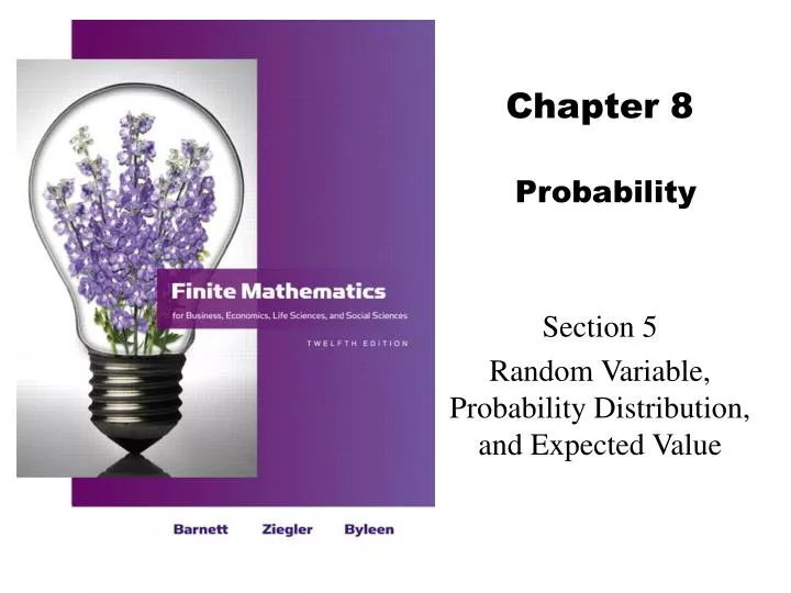
Chapter 8 Probability. Section 5 Random Variable, Probability Distribution, and Expected Value. Learning Objectives for Section 8.5 . Random Variable, Probability Distribution, and Expected Value. The student will be able to identify what is meant by a random variable.

E N D
Chapter 8Probability Section 5 Random Variable, Probability Distribution, and Expected Value
Learning Objectives for Section 8.5 Random Variable, Probability Distribution, and Expected Value • The student will be able to identify what is meant by a random variable. • The student will be able to create and use a probability distribution for a random variable. • The student will be able to compute the expected value of a random variable. • The student will be able to use the expected value of a random variable in decision-making. Barnett/Ziegler/Byleen Finite Mathematics 12e
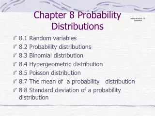
Random Variables A random variable is a function that assigns a numerical value to each simple event in a sample space S. If these numerical values are only integers (no fractions or irrational numbers), it is called a discrete random variable. Note that a random variable is neither random nor a variable - it is a function with a numerical value, and it is defined on a sample space. Barnett/Ziegler/Byleen Finite Mathematics 12e
Examples of Random Variables 1. A function whose range is the number of speeding tickets issued on a certain stretch of I 95 S. 2. A function whose range is the number of heads which appear when 4 dimes are tossed. 3. A function whose range is the number of passes completed in a game by a quarterback. These examples are all discrete random variables. Barnett/Ziegler/Byleen Finite Mathematics 12e
Probability Distributions The simple events in a sample space S could be anything: heads or tails, marbles picked out of a bag, playing cards. The point of introducing random variables is to associate the simple events with numbers, with which we can calculate. We transfer the probability assigned to elements or subsets of the sample space to numbers. This is called the probability distribution of the random variable X. It is defined as p(x) = P(X = x) Barnett/Ziegler/Byleen Finite Mathematics 12e
Example • A bag contains 2 black checkers and 3 red checkers. • Two checkers are drawn without replacement from this bag and the number of red checkers is noted. • Let X = number of red checkers drawn from this bag. • Determine the probability distribution of X and complete the table: Barnett/Ziegler/Byleen Finite Mathematics 12e
Example(continued) • Possible values of X are 0, 1, 2. (Why?) • p(x = 0) = P(black on first draw and black on second draw) = • Now, complete the rest of the table. Hint: Find p(x = 2) first, since it is easier to compute than p(x = 1) . Barnett/Ziegler/Byleen Finite Mathematics 12e
Example(continued) • Possible values of X are 0, 1, 2. (Why?) • p(x = 0) = P(black on first draw and black on second draw) = • Now, complete the rest of the table. Hint: Find p(x = 2) first, since it is easier to compute than p(x = 1) . Barnett/Ziegler/Byleen Finite Mathematics 12e
Properties of Probability Distribution Properties: 1. 0 <p(xi) < 1 2. The first property states that the probability distribution of a random variable X is a function which only takes on values between 0 and 1 (inclusive). The second property states that the sum of all the individual probabilities must always equal one. Barnett/Ziegler/Byleen Finite Mathematics 12e
X = number of customers in line waiting for a bank teller Verify that this describes a discrete random variable Example Barnett/Ziegler/Byleen Finite Mathematics 12e
X = number of customers in line waiting for a bank teller Verify that this describes a discrete random variable Solution: Variable X is discrete since its values are all whole numbers. The sum of the probabilities is one, and all probabilities are between 0 and 1 inclusive, so it satisfies the requirements for a probability distribution. ExampleSolution Barnett/Ziegler/Byleen Finite Mathematics 12e
Expected ValueExample Assume X = number of heads that show when tossing three coins. Sample space: HHH, HHT, HTH, THH, HTT, THT, TTH, TTT X = (0, 1, 1, 1, 2, 2, 2, 3) If you perform this experiment many times and average the number of heads, you would expect to find a number close to Barnett/Ziegler/Byleen Finite Mathematics 12e
Expected ValueExample (continued) Notice the outcomes of x = 1 and x = 2 occur three times each, while the outcomes x = 0 and x = 3 occur once each. We could calculate the average as Barnett/Ziegler/Byleen Finite Mathematics 12e
Expected Value of Random Variable The expected value of a random variable X is defined as How is this interpreted? If you perform an experiment thousands of times, record the value of the random variable every time, and average the values, you should get a number close to E(X). Barnett/Ziegler/Byleen Finite Mathematics 12e
Computing the Expected Value Step 1. Form the probability distribution of the random variable. Step 2. Multiply each image value of X, xi, by its corresponding probability of occurrence pi ; then add the results. Barnett/Ziegler/Byleen Finite Mathematics 12e
Application to Business A rock concert producer has scheduled an outdoor concert for Saturday, March 8. If it does not rain, the producer stands to make a $20,000 profit from the concert. If it does rain, the producer will be forced to cancel the concert and will lose $12,000 (rock star’s fee, advertising costs, stadium rental, etc.) The producer has learned from the National Weather Service that the probability of rain on March 8 is 0.4. A) Write a probability distribution that represents the producer’s profit. B) Find and interpret the producer’s “expected profit”. Barnett/Ziegler/Byleen Finite Mathematics 12e
Application to BusinessSolution (A) There are two possibilities: It rains on March 8, or it doesn’t. Let x represent the amount of money the producer will make. So, x can either be $20,000 (if it doesn’t rain) or x = -$12,000 (if it does rain). We can construct the following table: Barnett/Ziegler/Byleen Finite Mathematics 12e
Application to BusinessSolution (continued) (B) The expected value is interpreted as a long-term average. The number $7,200 means that if the producer arranged this concert many times in identical circumstances, he would be ahead by $7,200 per concert on the average. It does not mean he will make exactly $7,200 on March 8. He will either lose $12,000 or gain $20,000. Barnett/Ziegler/Byleen Finite Mathematics 12e