Download
1 / 71
720 likes | 870 Vues
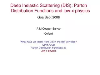
Parton distribution functions PDFs ZEUS Tutorial Dec 2006 A.M.Cooper-Sarkar Oxford What are they? How do we determine them? What are the uncertainties -experimental -model -theoretical

E N D
Parton distribution functions PDFs • ZEUS Tutorial Dec 2006 • A.M.Cooper-Sarkar • Oxford • What are they? • How do we determine them? • What are the uncertainties -experimental • -model • -theoretical • 4. Why are they important?
PDFs were first investigated in deep inelastic lepton-hadron scatterning -DIS Leptonic tensor - calculable 2 Lμν Wμν dσ~ Hadronic tensor- constrained by Lorentz invariance Et q = k – k’, Q2 = -q2 Px = p + q , W2 = (p + q)2 s= (p + k)2 x = Q2 / (2p.q) y = (p.q)/(p.k) W2 = Q2 (1/x – 1) Q2 = s x y Ee Ep s = 4 Ee Ep Q2 = 4 Ee E’ sin2θe/2 y = (1 – E’/Ee cos2θe/2) x = Q2/sy The kinematic variables are measurable
Completely generally the double differential cross-section for e-N scattering d2(e±N) = [ Y+ F2(x,Q2) - y2 FL(x,Q2) ± Y_xF3(x,Q2)], Y± = 1 ± (1-y)2 dxdy Leptonic part hadronic part F2, FL and xF3 are structure functionswhich express the dependence of the cross-section on the structure of the nucleon– The Quark-Parton model interprets these structure functions as related to the momentum distributions of quarks or partons within the nucleon AND the measurable kinematic variablex = Q2/(2p.q)is interpreted as the FRACTIONAL momentum of the incoming nucleon taken by the struck quark (xP+q)2=x2p2+q2+2xp.q ~ 0 for massless quarks and p2~0so x = Q2/(2p.q) The FRACTIONAL momentum of the incoming nucleon taken by the struck quark is the MEASURABLE quantity x e.g. for charged lepton beams F2(x,Q2) = Σi ei2(xq(x) + xq(x)) – Bjorken scaling FL(x,Q2) = 0 - spin ½ quarks xF3(x,Q2) = 0 - only γexchange However for neutrino beams xF3(x,Q2)= Σi (xq(x) - xq(x)) ~ valence quark distributions of various flavours
Consider electron muon scattering ds = 2pa2s [ 1 + (1-y)2] , for elastic eμ dy Q4 isotropic non-isotropic ds = 2pa2ei2 s [ 1 + (1-y)2] , for elastic eq, quark charge ei e dy Q4 d2s= 2pa2 s [ 1 + (1-y)2] Σiei2(xq(x) + xq(x)) for eN, where eq has c. of m. energy2 equal to xs, and q(x) gives probability that such a quark is in the Nucleon dxdy Q4 Now compare the general equation to the QPM prediction to obtain the results F2(x,Q2) = Σiei2(xq(x) + xq(x)) – Bjorken scaling FL(x,Q2) = 0 - spin ½ quarks xF3(x,Q2) = 0 - only γexchange
Consider n,n scattering: neutrinos are handed ds(n)= GF2 x s ds(n) = GF2 x s (1-y)2 Compare to the general form of the cross-section for n/n scattering via W+/- FL(x,Q2) = 0 xF3(x,Q2) = 2Σix(qi(x) - qi(x)) Valence F2(x,Q2) = 2Σix(qi(x) + qi(x)) Valence and Sea And there will be a relationship between F2eN and F2nN Also NOTE n,nbar scattering is FLAVOUR sensitive dy p dy p For nq (left-left) For n q (left-right) d2s(n) = GF2 s Σi [xqi(x) +(1-y)2xqi(x)] dxdy p For nN d2s(n) = GF2 s Σi [xqi(x) +(1-y)2xqi(x)] dxdy p For nN Clearly there are antiquarks in the nucleon 3 Valence quarks plus a flavourless qq Sea m- W+ can only hit quarks of charge -e/3 or antiquarks -2e/3 n W+ u d s(np)~ (d + s) + (1- y)2 (u + c) s(np) ~ (u + c) (1- y)2 + (d + s) q = qvalence +qsea q = qsea qsea= qsea
So in n,nbar scattering the sums over q, qbar ONLY contain the appropriate flavours BUT- high statistics n,nbar data are taken on isoscalar targets e.g. Fe = (p + n)/2 = N d in proton = u in neutron u in proton = d in neutron GLS sum rule Total momentum of quarks A TRIUMPH (and 20 years of understanding the c c contribution)
Bjorken scaling is broken – ln(Q2) Note strong rise at small x
QCD improves the Quark Parton Model What if or x x Pqq Pgq y y Before the quark is struck? Pqg Pgg y > x, z = x/y So F2(x,Q2) = Σi ei2(xq(x,Q2) + xq(x,Q2)) in LO QCD The theory predicts the rate at which the parton distributions (both quarks and gluons) evolve with Q2- (the energy scale of the probe) -BUT it does not predict their shape The DGLAP parton evolution equations
Note q(x,Q2) ~ αs lnQ2, but αs(Q2)~1/lnQ2, so αs lnQ2 is O(1), so we must sum all terms What if higher orders are needed? αsn lnQ2n Leading Log Approximation x decreases from ss(Q2) target to probe xi-1> xi > xi+1…. pt2 of quark relative to proton increases from target to probe pt2i-1 < pt2i < pt2i+1 Dominant diagrams have STRONG pt ordering Pqq(z) = P0qq(z) + αs P1qq(z) +αs2 P2qq(z) LO NLO NNLO F2 is no longer so simply expressed in terms of partons - convolution with coefficient functions is needed – but these are calculable in QCD
How do we determine Parton Distribution Functions ? Parametrise the parton distribution functions (PDFs) at Q20 (~1-7 GeV2)- Use QCD to evolve these PDFs to Q2 >Q20 Construct the measurable structure functions and cross-sections by convoluting PDFs with coefficient functions: make predictions for ~2000 data points across the x,Q2 plane- Perform χ2 fit to the data Who? Alekhin, CTEQ, MRST, GGK, Botje, H1, ZEUS, GRV, BFP, … http://durpdg.dur.ac.uk/hepdata/ Formalism NLO DGLAP MSbar factorisation Q02 functional form @ Q02 sea quark (a)symmetry etc. fi (x,Q2) fi (x,Q2) αS(MZ ) Data DIS (SLAC, BCDMS, NMC, E665, CCFR, H1, ZEUS, … ) Drell-Yan (E605, E772, E866, …) High ET jets (CDF, D0) W rapidity asymmetry (CDF) N dimuon (CCFR, NuTeV) etc. LHAPDFv5
The DATA – the main contribution is DIS data Terrific expansion in measured range across the x, Q2 plane throughout the 90’s HERA data Pre HERA fixed target p,D NMC, BDCMS, E665 and ,bar Fe CCFR We have to impose appropriate kinematic cuts on the data so as to remain in the region when the NLO DGLAP formalism is valid • Q2 cut : Q2 > few GeV2 so that perturbative QCD is applicable- αs(Q2) small • W2 cut: W2 > 20 GeV2 to avoid higher twist terms- usual formalism is leading twist • x cut: to avoid regions where ln(1/x) resummation (BFKL) and non-linear effects may be necessary
Need to extend the formalism? Optical theorem 2 The handbag diagram- QPM Im QCD at LL(Q2) Ordered gluon ladders (αsn lnQ2 n) NLL(Q2) one rung disordered αsn lnQ2 n-1 ? BUT what about completely disordered Ladders? at small x there may be a need for BFKLln(1/x) resummation? And what about Higher twist diagrams ? Are they always subdominant? Important at high x, low Q2
The strong rise in the gluon density at small-x leads to speculation that there may be a need for non-linear equations?- gluons recombining gg→g Non-linear fan diagrams form part of possible higher twist contributions at low x
The CUTS In practice it has been amazing how low in Q2 the standard formalism still works- down to Q2 ~ 1 GeV2 : cut Q2 > 2 GeV2 is typical It has also been surprising how low in x – down to x~ 10-5 : no x cut is typical Nevertheless there are doubts as to the applicability of the formalism at such low-x.. there could beln(1/x) corrections and/or non-linear high density corrections for x < 5 10 -3
The form of the parametrisation Parametrise the parton distribution functions (PDFs) at Q20 (~1-7 GeV2) Parameters Ag, Au, Ad are fixed through momentum and number sum rules– explain other parameters may be fixed by model choices- Model choices Form of parametrization at Q20, value ofQ20,, flavour structure of sea, cuts applied, heavy flavour scheme → typically ~15 parameters Use QCD to evolve these PDFs to Q2 >Q20 Construct the measurable structure functions by convoluting PDFs with coefficient functions: make predictions for ~2000 data points across the x,Q2 plane Perform χ2 fit to the data xuv(x) =Auxau (1-x)bu (1+ εu√x + γu x) xdv(x) =Adxad (1-x)bd (1+ εd√x + γdx) xS(x) =Asx-λs (1-x)bs (1+ εs√x + γsx) xg(x) =Agx-λg(1-x)bg (1+ εg√x + γgx) These parameters control the low-x shape These parameters control the middling-x shape These parameters control the high-x shape Alternative form for CTEQ xf(x) = A0xA1(1-x)A2 eA3x (1+eA4x)A5 The fact that so few parameters allows us to fit so many data points established QCD as the THEORY OF THE STRONG INTERACTION and provided the first measurements of s (as one of the fit parameters)
Where is the information coming from? • Fixed target e/μ p/D data from NMC, BCDMS, E665, SLAC • F2(e/p)~ 4/9 x(u +ubar) +1/9x(d+dbar) + 4/9 x(c +cbar) +1/9x(s+sbar) • F2(e/D)~5/18 x(u+ubar+d+dbar) + 4/9 x(c +cbar) +1/9x(s+sbar) • Also use ν, νbar fixed target data from CCFR(Beware Fe target needs corrections) • F2(ν,νbar N) = x(u +ubar + d + dbar + s +sbar + c + cbar) • xF3(ν,νbar N) = x(uv + dv ) (provided s = sbar) • Valence information for 0< x < 1 • Can get ~4 distributions from this: e.g. u, d, ubar, dbar – but need assumptions • like q=qbar for all flavours, sbar = 1/4 (ubar+dbar), dbar = ubar (wrong!) and need heavy quark treatment. • (Not going to cover flavour structure in this talk) • Note gluon enters only indirectly via DGLAP equations for evolution Assuming u in proton = d in neutron – strong-isospin
Low-x – within conventional NLO DGLAP Before the HERA measurements most of the predictions for low-x behaviour of the structure functions and the gluon PDF were wrong HERA ep neutral current (γ-exchange) data give much more information on the sea and gluon at small x….. xSea directly from F2, F2 ~ xq xGluon from scaling violations dF2 /dlnQ2 – the relationship to the gluon is much more direct at small-x, dF2/dlnQ2 ~ Pqgxg
Low-x t = ln Q2/2 Gluon splitting functions become singular αs ~ 1/ln Q2/2 At small x, small z=x/y A flat gluon at low Q2 becomes very steep AFTER Q2 evolution AND F2 becomes gluon dominated F2(x,Q2) ~ x -λs, λs=λg -ε xg(x,Q2) ~ x -λg
High Q2 HERA data HERA data have also provided information at high Q2→ Z0 and W+/- become as important as γexchange → NC and CC cross-sections comparable For NC processes F2= i Ai(Q2) [xqi(x,Q2) + xqi(x,Q2)] xF3= iBi(Q2) [xqi(x,Q2) - xqi(x,Q2)] Ai(Q2) = ei2 – 2 eivi vePZ + (ve2+ae2)(vi2+ai2) PZ2 Bi(Q2) = – 2 eiai ae PZ + 4ai ae vi ve PZ2 PZ2 = Q2/(Q2 + M2Z) 1/sin2θW a new valence structure function xF3 due to Z exchange is measurable from low to high x- on a pure proton target → no heavy target corrections- no assumptions about strong isospin running at HERA-II is already improving this measurement
CC processes give flavour information d2(e+p) = GF2 M4W [x (u+c) + (1-y)2x (d+s)] d2(e-p) = GF2 M4W [x (u+c) + (1-y)2x (d+s)] dxdy 2x(Q2+M2W)2 dxdy 2x(Q2+M2W)2 uv at high x dv at high x MW information Measurement of high-x dvon a pure proton target d is not well known because u couples more strongly to the photon. Historically information has come from deuterium targets –but even Deuterium needs binding corrections. Open questions: does u in proton = d in neutron?, does dvalence/uvalence 0, as x 1?
Parton distributions are transportable to other processes Accurate knowledge of them is essential for calculations of cross-sections of any process involving hadrons. Conversely, some processes have been used to get further information on the PDFs E.G DRELL YAN – p N →μ+μ- X, via q qbar →μ+μ-, gives information on the Sea Asymmetry between pp →μ+μ- X and pn→μ+μ- X gives more information on dbar - ubar difference W PRODUCTION- p pbar → W+(W-) X, via u dbar → W+, d ubar → W- gives more information on u, d differences PROMPT g - p N → g X, via g q → g q gives more information on the gluon (but there are current problems concerning intrinsic pt of initial partons) HIGH ET INCLUSIVE JET PRODUCTION – p p → jet + X, via g g, g q, g qbar subprocesses gives more information on the gluon
New millenium PDFs With uncertainty estimates –Valence distributions evolve slowly Sea/Gluon distributions evolve fast
So how certain are we? First, some quantitative measure of the progress made over 20 years of PDF fitting ( thanks to Wu-ki Tung)
To reveal the difference in both large and small x regions To view small and large x in one plot The u quark LO fits to early fixed-target DIS data
Gluon HERA
Gluon More recent fits with HERA data Tev jet data Does gluon go negative at small x and low Q?seeMRST PDFs
Heavy quarks Heavy quark distributions in fits are dynamically generated from g→c cbar Results dependon the “scheme” chosen to handle heavy quark effects in pQCD–fixed-flavor-number (FFN) vs. variable-flavor-number (VFN) schemes.
Modern analyses assess PDF uncertainties within the fit Clearly errors assigned to the data points translate into errors assigned to the fit parameters -- and these can be propagated to any quantity which depends on these parameters— the parton distributions or the structure functions and cross-sections which are calculated from them < б2F > = Σj Σk ∂ F Vjk ∂ F ∂ pj ∂ pk The errors assigned to the data are both statistical and systematic and for much of the kinematic plane the size of the point-to-point correlated systematic errors is ~3 times the statistical errors.
What are the sources of correlated systematic errors? Normalisations are an obvious example BUT there are more subtle cases- e.g. Calorimeter energy scale/angular resolutions can move events between x,Q2 bins and thus change the shape of experimental distributions Vary the estimate of the photo-production background Vary energy scales in different regions of the calorimeter Vary position of the RCAL halves Why does it matter?
Treatment of correlated systematic errors χ2 = Σi [ FiQCD (p) – Fi MEAS]2 (siSTAT)2+(ΔiSYS)2 Errors on the fit parameters, p, evaluated fromΔχ2 = 1, THIS IS NOT GOOD ENOUGH ifexperimental systematic errors are correlated between data points- χ2 = Σi Σj [ FiQCD(p) – FiMEAS] Vij-1 [ FjQCD(p) – FjMEAS] Vij = δij(бiSTAT)2 + ΣλΔiλSYSΔjλSYS Where ΔiλSYS is the correlated error on point i due to systematic error sourceλ It can be established that this is equivalent to χ2 = Σi [ FiQCD(p) –ΣλslDilSYS – FiMEAS]2 + Σsl2 (siSTAT) 2 Wheresλare systematic uncertainty fit parameters of zero mean and unit variance This has modified the fit prediction by each source of systematic uncertainty CTEQ, ZEUS, H1, MRST have all adopted this form of χ2 – but use it differently in the OFFSET and HESSIAN methods …hep-ph/0205153
How do experimentalists usually proceed: OFFSET method • Perform fit without correlated errors (sλ = 0) for central fit • Shift measurement to upper limit of one of its systematic uncertainties (sλ = +1) • Redo fit, record differences of parameters from those of step 1 • Go back to 2, shift measurement to lower limit (sλ= -1) • Go back to 2, repeat 2-4 for next source of systematic uncertainty • Add all deviations from central fit in quadrature (positive and negative deviations added in quadrature separately) • This method does not assume that correlated systematic uncertainties are Gaussian distributed • Fortunately, there are smart ways to do this (Pascaud and Zomer LAL-95-05, Botje hep-ph-0110123) • ZEUS uses the OFFSET method
There are other ways to treat correlated systematic errors- HESSIAN method (covariance method) Allow sλ parameters to vary for the central fit. If we believe the theory why not let it calibrate the detector(s)?Effectively the theoretical prediction is not fitted to the central values of published experimental data, but allows these data points to move collectively according to their correlated systematic uncertainties The fit determines the optimal settings for correlated systematic shifts such that the most consistent fit to all data sets is obtained. In a global fit the systematic uncertainties of one experiment will correlate to those of another through the fit The resulting estimate of PDF errors is much smaller than for the Offset method for Δχ2 = 1 We must be very confident of the theoryto trust it for calibration– but more dubiously we must be very confident of the model choices we made in setting boundary conditions H1 uses the HESSIAN method with Δχ2 =1 CTEQ uses the HESSIAN method with increased Δχ2=100 MRST uses a compromise between HESSIAN and quadratic with increased Δχ2=50
WHY? - In practice there are problems. Some data sets incompatible/only marginally compatible? One could restrict the data sets to those which are sufficiently consistent that these problems do not arise – (H1, GKK, Alekhin) But one loses information since partons need constraints from many different data sets – no-one experiment has sufficient kinematic range / flavour info. To illustrate: the χ2 for the MRST global fit is plotted versus the variation of a particular parameter (αs ). The individual χ2e for each experiment is also plotted versus this parameter in the neighbourhood of the global minimum. Each experiment favours a different value of. αs PDF fitting is a compromise. Can one evaluate acceptable ranges of the parameter value with respect to the individual experiments?
illustration foreigenvector-4 CTEQ look at eigenvector combinations of their parameters rather than the parameters themselves. They determine the 90% C.L. bounds on the distance from the global minimum from P(χe2, Ne) dχe2 =0.9 for each experiment Distance This leads them to suggest a modification of the χ2 tolerance, Δχ2 = 1, with which errors are evaluated such that Δχ2 = T2, T = 10. Why? Pragmatism. The size of the tolerance T is set by considering the distances from the χ2 minima of individual data sets from the global minimum for all the eigenvector combinations of the parameters of the fit. All of the world’s data sets must be considered acceptable and compatible at some level, even if strict statistical criteria are not met, since the conditions for the application of strict statistical criteria, namely Gaussian error distributions are also not met. One does not wish to lose constraints on the PDFs by dropping data sets, but the level of inconsistency between data sets must be reflected in the uncertainties on the PDFs.
Compare gluon PDFs for Hessian and Offset methods for the ZEUS fit analysis Offset method Hessian method T=1 Hessian method T=7 The Hessian method gives comparable size of error band as the Offset method, when the tolerance is raised to T ~ 7– (similar ball park to CTEQ, T=10) Note this makes the error band large enough to encompass reasonable variations of model choice. (For the ZEUS global fit √2N=50, where N is the number of degrees of freedom)
Aside on model choices We trust NLO QCD– but are we sure about every choice which goes into setting up the boundary conditions for QCD evolution? – form of parametrization etc. The statistical criterion for parameter error estimation within a particular hypothesis is Δχ2 = T2 = 1. But for judging the acceptability of an hypothesis the criterion is that χ2 lie in the range N ±√2N, where N is the number of degrees of freedom There are many choices, such as the form of the parametrization at Q20, the value of Q02 itself, the flavour structure of the sea, etc., which might be considered as superficial changes of hypothesis, but the χ2 change for these different hypotheses often exceeds Δχ2=1, while remaining acceptably within the range N ±√2N. In this case the model error on the PDF parameters usually exceeds the experimental error on the PDF, if this has been evaluated using T=1, with the Hessian method.
If the experimental errors have been estimated by the Hessian method with T=1, then the model errors are usually larger. Use of restricted data sets also results in larger model errors. Hence total error (model + experimental) can end up being in the same ball park as the Offset method ( or the Hessian method with T ~ 7-10). Comparison of ZEUS (Offset) and H1(Hessian, T=1) gluon distributions – Yellow band (total error) of H1 comparable to red band (total error) of ZEUS Swings and roundabouts
Last remarks on the Hessian versus the Offset method • It may be dangerous to let the QCD fit determine the optimal values for the systematic shift parameters. • Comparison of sλ values determined using a Hessian NLO QCD PDF fit to ZEUS and H1 data • with sλ values determined using a ‘theory-free’ Hessian fit to combine the data.
The general trend of PDF uncertainties is that The u quark is much better known than the d quark The valence quarks are much better known than the gluon at high-x The valence quarks are poorly known at small-x but they are not important for physics in this region The sea and the gluon are well known at low-x The sea is poorly known at high-x, but the valence quarks are more important in this region The gluon is poorly known at high-x And it can still be very important for physics e.g.– high ET jet xsecn need to tie down the high-x gluon
Good news: PDF uncertainties will decrease before LHC comes on lineHERA-II and Tevatron Run-II will improve our knowledge Example- decrease in gluon PDF uncertainty from using ZEUS jet data in ZEUS PDF fit. Direct* Measurement of the Gluon Distribution ZEUS jet data much more accurate than Tevatron jet data- small energy scale uncertainties
After jets Before jets Also gives a nice measurement of αs(MZ) = 0.1183 ± 0.0028 (exp) ± 0.0008 (model) From simultaneous fit of αs(MZ) & PDF parameters And correspondingly the contribution of the uncertainty onαs(MZ) to the uncertainty on the PDFs is much reduced
Why are PDF’s important At the LHC high precision (SM and BSM) cross section predictions require precision Parton Distribution Functions (PDFs) How do PDF uncertainties affect discovery physics? BSM EXAMPLE--- high ET jets Where new physics could show up e.g...contact interactions/extra dimensions SM EXAMPLE----W/Z cross-section as ‘standard candle’ calibration processes
fa pA x1 • where X=W, Z, D-Y, H, high-ET jets, prompt-γ • and is known • to some fixed order in pQCD and EW • in some leading logarithm approximation (LL, NLL, …) to all orders via resummation ^ pB x2 fb X HERA and the LHC- transporting PDFs to hadron-hadron cross-sections QCD factorization theorem for short-distance inclusive processes
Connection of HERA data to the LHC LHC is a low-x machine (at least for the early years of running) Low-x information comes from evolving the HERA data Is NLO (or even NNLO) DGLAP good enough? The QCD formalism may need extending at small-x BFKL ln(1/x) resummation High density non-linear effects etc But let’s stick to the conventional NLO DGLAP and see what HERA has achieved..
What has HERA data ever done for us? W+ W- Z Pre-HERA W+/W-/Z and W+/- → lepton+/- rapidity spectra ~ ± 15% uncertainties ! Why? Because the central rapidity range AT LHC is at low-x (5 10-4 to 5 10-2) NO WAY to use these cross-sections as standard candles Lepton+ Lepton-
W+ W- Z Lepton+ Lepton- Post-HERA W+/W-/Z and W+/- → lepton+/- rapidity spectra ~ ± 5% uncertainties ! Why? Because there has been a tremendous improvement in our knowledge of the low-x glue and thus of the low-x sea
Pre-HERA sea and glue distributions Post HERA sea and glue distributions BUT BEWARE! If the NLO DGLAP formalism we are using at low-x is wrong/incomplete it will show up right in the measurable rapidity range for W/Z production at the LHC
Example of how PDF uncertainties matter for BSM physics– Tevatron jet data were originally taken as evidence for new physics-- i These figures show inclusive jet cross-sections compared to predictions in the form (data - theory)/ theory Something seemed to be going on at the highest E_T And special PDFs like CTEQ4/5HJ were tuned to describe it better- note the quality of the fits to the rest of the data deteriorated. But this was before uncertainties on the PDFs were seriously considered