Download
1 / 23
230 likes | 399 Vues
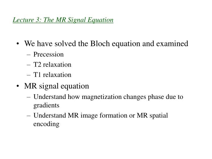
Lecture 3: The MR Signal Equation. We have solved the Bloch equation and examined Precession T2 relaxation T1 relaxation MR signal equation Understand how magnetization changes phase due to gradients Understand MR image formation or MR spatial encoding. Complex transverse magnetization: m.

E N D
Lecture 3: The MR Signal Equation • We have solved the Bloch equation and examined • Precession • T2 relaxation • T1 relaxation • MR signal equation • Understand how magnetization changes phase due to gradients • Understand MR image formation or MR spatial encoding
Complex transverse magnetization: m m is complex. m =Mx+iMy Re{m} =Mx Im{m}=My This notation is convenient: It allows us to represent a two element vector as a scalar. Im m My Re Mx
Inhomogeneous Object - Nonuniform field. Now we get much more general. Before, M(t) was constant in space and so no spatial variable was needed to describe it. Now, we let it vary spatially. We also let the z component of the B field vary in space. This variation gives us a new phase term, or perhaps a more general one than we have seen before.
Transverse Magnetization Equation We can number the terms above 1-4 1. - variation in proton density 2. - spatial variation due to T2 3. - rotating frame frequency - “carrier” frequency of signal 4. - spins will precess at differential frequency according to the gradient they experience (“see”).
Transverse Magnetization Equation - spins will precess at differential frequency according to the gradient they “see”. Phase is the integral of frequency. Thus, gradient fields allow us to change the frequency and thus the phase of the signal as a function of its spatial location. Let’s study this general situation under several cases, from the specific to the general.
The Static Gradient Field In a static (non-time-varying) gradient field, for example in x, Plugging into solution (from 2 slides ago) and simplifying yields
The Static Gradient Field Now, let the gradient field have an arbitrary direction. But the gradient strength won’t vary with time. Using dot notation, Takes into account the effects of both the static magnetic and gradient fields on the magnetization gives
Time –Varying Gradient Solution (Non-static) . We can make the previous expression more general by allowing the gradients to change in time. If we do, the integral of the gradient over time comes back into the above equation.
Receiving the signal Let’s assume we now use a receiver coil to “read” the transverse magnetization signal We will use a coil that has a flat sensitivity pattern in space. Is this a good assumption? - Yes, it is a good assumption, particularly for the head and body coils. Then the signal we receive is an integration of over the three spatial dimensions.
Receiving the signal (2) Let’s simplify this: 1) Ignore T2 for now; it will be easy to add later. 2) Assume 2D imaging. (Again, it will be easy to expand to 3 later.) 3) Demodulate to baseband. i.e. zo slice thickness z S(t) is complex.
Receiving the signal (3) S(t) is complex. Then, 3) Demodulate to baseband. i.e. end goal
Gx(t) and Gy(t) Now consider Gx(t) and Gy(t) only. Deja vu strikes, but we push on! Let
kxand ky related to t Let As we move along in time (t) in the signal, we simply change where we are in kx, ky (dramatic pause as students inch to edge of seats...)
kxand ky related to t (2) x kx, y kyare reciprocal variables. x,y are in cm, kx,kyare in cycles/cm or cycles/mm Remarks: 1) S(t), our signal, are values of M along a trajectory in F.T. space. - (called k-space in MR literature) 2) Integral of Gx(t), Gy(t), controls the k-space trajectory. 3) To image m(x,y), acquire set of S(t) to cover k-space and apply inverse Fourier Transform.
What is ? Spatial Encoding Summary Receiver detects signal Consider phase. Frequency is time rate of change of phase. So
Spatial Encoding Summary But So Expanding, We control frequency with gradients. So,
Complex Demodulation • The signal is complex. How do we realize this? • In ultrasound, like A.M. radio, we use envelope detection, which is phase-insensitive. • In MR, phase is crucial to detecting position. Thus the signal is complex. We must receive a complex signal. How do we do this when voltage is a real signal?
Complex Demodulation sr(t) is a complex signal, but our receiver voltage can only read a single voltage at a time. sr(t) is a useful concept, but in the real world, we can only read a real signal. How do we read off the real and imaginary components of the signal, sr(t)? Complex receiver signal ( mathematical concept) The quantity s(t) or another representation, is what we are after. We can write s(t) as a real and imaginary component, I(t) and Q(t)
Complex Demodulation An A/D converter reading the coil signal would read the real portion of sr(t), the physical signal sp(t)
Complex Demodulation Inphase: I(t) X Low Pass Filter sp(t) cos(w0t) X Low Pass Filter Quadrature: Q(t) sin(w0t) Let’s next look at the signal right after the multipliers. We can consider the modulation theorem or trig identities.
Complex Demodulation Inphase: I(t) X Low Pass Filter sp(t) cos(w0t) X Low Pass Filter Quadrature: Q(t) sin(w0t)
Complex Demodulation Inphase: I(t) X Low Pass Filter sp(t) cos(w0t) X Low Pass Filter Quadrature: Q(t) sin(w0t)
Complex Demodulation The low pass filters have an impulse response that removes the frequency component at 2w0 We can also consider them to have gain to compensate for the factor ½.