Download
1 / 23
230 likes | 391 Vues
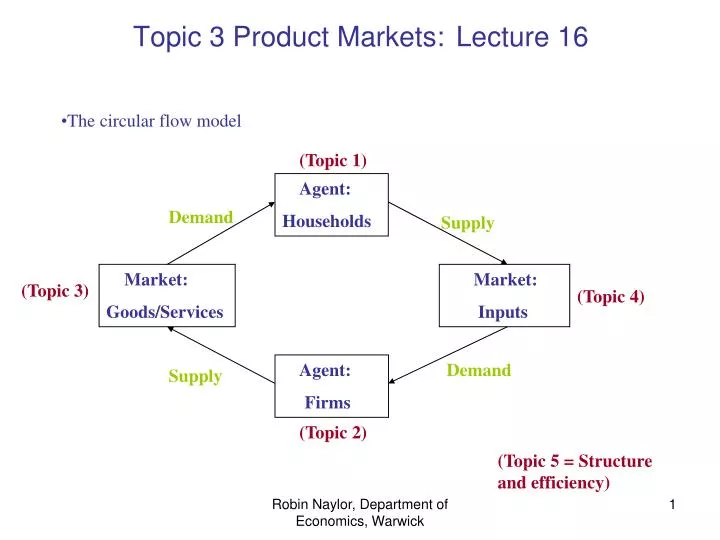
Topic 3 Product Markets: Lecture 16. The circular flow model. (Topic 1). Agent: Households. Demand. Supply. Market: Goods/Services. Market: Inputs. (Topic 3). (Topic 4). Agent: Firms. Demand. Supply. (Topic 2). (Topic 5 = Structure and efficiency).

E N D
Topic 3 Product Markets:Lecture 16 • The circular flow model (Topic 1) Agent: Households Demand Supply Market: Goods/Services Market: Inputs (Topic 3) (Topic 4) Agent: Firms Demand Supply (Topic 2) (Topic 5 = Structure and efficiency) Robin Naylor, Department of Economics, Warwick
Topic 3 :Lecture 16 Markets differ by nature/extent of competition. So far, we have assumed (at least implicitly) that there is just one firm in the market, confronting the entire market demand: a monopolist. Now consider the extreme opposite case of ‘perfect competition’ – then we’ll look at perhaps more realistic intermediate cases. Robin Naylor, Department of Economics, Warwick
Topic 3 :Lecture 16 Perfect competition All (the very many) firms are assumed identical and will set the same price (each is a price-taker) because: a firm cannot charge more than the competitive market price (assuming homogeneous goods and perfect information) a firm cannot charge less than the market price (free entry means that all firms will just break even at the market price) each firm is so ‘small’ it does not affect market price. Hence: Robin Naylor, Department of Economics, Warwick
Topic 3 :Lecture 16 Perfect competition Consider the individual firm i: p pc pc = d x The firm is a price-taker at the market price. Demand is perfectly elastic. Robin Naylor, Department of Economics, Warwick
Topic 3 :Lecture 16 Perfect competition p pc pc = d = mr x Because the firm does not have to reduce price to sell an extra unit (because it is so ‘small’), the marginal revenue is equal to price. Hence, p = d = mr. Robin Naylor, Department of Economics, Warwick
Topic 3 Lecture 16 This diagram is the same as that in Lecture 15 Slide 2, except that we now have d=mr=p as perfectly elastic. SATC p SMC SAVC pc pc = d = mr x What is the firm’s chosen output level? Robin Naylor, Department of Economics, Warwick
Topic 3 Lecture 16 SATC p SMC SAVC pc pc = d = mr x Suppose market price rises: now what is the firm’s chosen output? What can you say about the firm’s (short-run) supply curve? Robin Naylor, Department of Economics, Warwick
Topic 3 Lecture 16 SMC SATC p SAVC pc pc = d = mr x Suppose market price falls: now what is the firm’s chosen output? What can you say about the firm’s (short-run) supply curve? Robin Naylor, Department of Economics, Warwick
Topic 3 Lecture 16 SATC p SMC = s SAVC pc pc = d = mr x Suppose market price falls further: now what is the firm’s chosen output? What can you say about the firm’s (short-run) supply curve? Robin Naylor, Department of Economics, Warwick
Topic 3 :Lecture 16 Perfect competition Now consider the long run and also where market price comes from: p p S Market price is where market supply meets market demand. Market demand is exogenous. What determines market supply? The market price determines the demand curve faced by the individual firm. And hence also mr. pc = d = mr pc D x Xc X Robin Naylor, Department of Economics, Warwick
Topic 3 :Lecture 16 Perfect competition Here we add the firm’s cost curves (and hence its supply curve): for the long run. p p S lmc = s lac Can you say where this market supply curve, S, comes from? pc pc = d = mr D x Xc X Robin Naylor, Department of Economics, Warwick
Topic 3 :Lecture 16 Perfect competition This industry is in equilibrium: why? Define and Explain Recall that we are assuming that all firms are identical. So this is the ‘representative firm’. p p lmc = s lac This is the long-run industry supply curve for a fixed number of firms, n. pc pc = d = mr D x* x Xc = nx* X Robin Naylor, Department of Economics, Warwick
Topic 3 :Lecture 16 Perfect competition We now want to derive the long-run industry supply curve when the number of firms is not fixed but is allowed to vary so as to yield industry equilibrium, whatever the level of demand. p p lmc = s lac Suppose there is an (exogenous) increase in the level of market demand. pc pc = d = mr D x* x Xc = nx* X Robin Naylor, Department of Economics, Warwick
Topic 3 :Lecture 16 Perfect competition We want to derive now the long-run industry supply curve when the number of firms is not fixed but is allowed to vary so as to yield industry equilibrium, whatever the level of demand. p p lmc = s lac pc pc = d = mr D’ D x* x Xc = nx* X The initial effect is that market price will rise so that supply by the n firms is equal to demand. Each firm is producing increased output. What can you say about profits? And industry equilibrium? Robin Naylor, Department of Economics, Warwick
Topic 3 :Lecture 16 Perfect competition We want to derive now the long-run industry supply curve when the number of firms is not fixed but is allowed to vary so as to yield industry equilibrium, whatever the level of demand. p p lmc = s lac pc pc = d = mr D’ D x* x Xc = nx* X New firms will enter the industry (why?). How do we show this in the diagram? Robin Naylor, Department of Economics, Warwick
Topic 3 :Lecture 16 Perfect competition We want to derive now the long-run industry supply curve when the number of firms is not fixed but is allowed to vary so as to yield industry equilibrium, whatever the level of demand. p p lmc = s lac pc pc = d = mr D’ D x* x Xc = nx* Xc = (n+E)x* X New firms enter the industry. Where does this process take us? (What are we assuming about new firms and about industry costs?) Robin Naylor, Department of Economics, Warwick
Topic 3 :Lecture 16 Perfect competition We want to derive now the long-run industry supply curve when the number of firms is not fixed but is allowed to vary so as to yield industry equilibrium, whatever the level of demand. p p lmc = s lac pc pc = d = mr D’ D x* x Xc = nx* Xc = (n+E)x* X So, in the new equilibrium following the increase in demand: market output is higher; price is unchanged; each of the original firms has returned to its original actions, there are more firms. Robin Naylor, Department of Economics, Warwick
Topic 3 :Lecture 16 Perfect competition We want to derive now the long-run industry supply curve when the number of firms is not fixed but is allowed to vary so as to yield industry equilibrium, whatever the level of demand. p p lmc = s lac LRSS pc pc = d = mr D’ D x* x Xc = nx* Xc = (n+E)x* X What does the long-run industry supply curve look like? It is perfectly elastic. Essentially, this is because new firms can enter the market without needing the market price to remain higher than at the initial equilibrium. Robin Naylor, Department of Economics, Warwick
Topic 3 :Lecture 16 Perfect competition What does the long-run industry supply curve look like when new firms are not equally efficient, but when – instead – new firms are less efficient than the original incumbents? p p lmci = s lac pc pc = d = mr We are assuming that firms are not equally efficient. So this is the ‘marginal firm,’ initially. D’ D xi x Xc X Originally, there is a marginal firm, i, which just breaks even. Then demand shifts and each of the original n firms raises output. So firm i now makes a supernormal profit. Then what happens? Robin Naylor, Department of Economics, Warwick
Topic 3 :Lecture 16 Perfect competition What does the long-run industry supply curve look like when new firms are not equally efficient, but when – instead – new firms are less efficient than the original incumbents? p p lmci = s lac b LRSS?? pc a pc = d = mr D’ D xi x Xc X New firms enter: the number is now n+E. Could this be the new equilibrium? Robin Naylor, Department of Economics, Warwick
Topic 3 :Lecture 16 Perfect competition What does the long-run industry supply curve look like when new firms are not equally efficient, but when – instead – new firms are less efficient than the original incumbents? lacj p p lmci,j = s laci b LRSS?? pc a pc = d = mr D’ D x* x Xc = nx* Xc = (n+E)x* X Point ‘b’ will be an equilibrium if . . . ? And so the LRSS is where? Robin Naylor, Department of Economics, Warwick
Topic 3 :Lecture 16 Perfect competition What does the long-run industry supply curve look like when new firms are not equally efficient, but when – instead – new firms are less efficient than the original incumbents? lacj p p lmci,j = s laci LRSS?? b pc a pc = d = mr D’ D x* x Xc = nx* Xc = (n+E)x* X Point ‘b’ will be an equilibrium if . . . ? And so the LRSS is where? And the intuition? What else would make the long-run industry supply curve upward-sloping (imperfectly elastic)? Robin Naylor, Department of Economics, Warwick
Topic 2: Lecture 16 • Now read B&B 4th Ed., pp. 328-341, 345-352, 353-366. • Note that in B&B (eg p. 337) a distinction is drawn between 2 types of short-run fixed cost: • Sunk Fixed Costs and • Non-sunk Fixed Costs. • I’m not making that distinction in lectures as, for simplicity, I’m assuming that all Fixed Costs are Sunk (i.e., unavoidable even if output is zero). Robin Naylor, Department of Economics, Warwick