Artificial Neural Networks Notes based on Nilsson and Mitchell’s Machine learning

1. Artificial Neural Networks Notes based on Nilsson and Mitchell’s Machine learning

2. Outline • Perceptrons (LTU) • Gradient descent • Multi-layer networks • Backpropagation

3. Biological Neural Systems • Neuron switching time : > 10-3 secs • Number of neurons in the human brain: ~1010 • Connections (synapses) per neuron : ~104–105 • Face recognition : 0.1 secs • High degree of parallel computation • Distributed representations

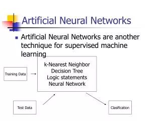
4. Properties of Artificial Neural Nets (ANNs) • Many simple neuron-like threshold switching units • Many weighted interconnections among units • Highly parallel, distributed processing • Learning by adaptation of the connection weights

5. Appropriate Problem Domains for Neural Network Learning • Input is high-dimensional discrete or real-valued (e.g. raw sensor input) • Output is discrete or real valued • Output is a vector of values • Form of target function is unknown • Humans do not need to interpret the results (black box model)

6. General Idea • A network of neurons. Each neuron is characterized by: • number of input/output wires • weights on each wire • threshold value • These values are not explicitly programmed, but they evolve through a training process. • During training phase, labeled samples are presented. If the network classifies correctly, no weight changes. Otherwise, the weights are adjusted. • backpropagation algorithm used to adjust weights.

7. ALVINN (Carnegie Mellon Univ) Automated driving at 70 mph on a public highway Camera image 30 outputs for steering 30x32 weights into one out of four hidden unit 4 hidden units 30x32 pixels as inputs

8. Another Example • NETtalk – Program that learns to pronounce English text. (Sejnowski and Rosenberg 1987). • A difficult task using conventional programming models. • Rule-based approaches are too complex since pronunciations are very irregular. • NETtalk takes as input a sentence and produces a sequence of phonemes and an associated stress for each letter.

9. NETtalk A phoneme is a basic unit of sound in a language. Stress – relative loudness of that sound. Because the pronunciation of a single letter depends upon its context and the letters around it, NETtalk is given a seven character window. Each position is encoded by one of 29 symbols, (26 letters and 3 punctuations.) Letter in each position activates the corresponding unit.

10. NETtalk The output units encode phonemes using 21 different features of human articulation. Remaining five units encode stress and syllable boundaries. NETtalk also has a middle layer (hidden layer) that has 80 hidden units and nearly 18000 connections (edges). NETtalk is trained by giving it a 7 character window so that it learns the pronounce the middle character. It learns by comparing the computed pronunciation to the correct pronunciation.

11. Handwritten character recognition • This is another area in which neural networks have been successful. • In fact, all the successful programs have a neural network component.

12. x1 x2 xn Threshold Logic Unit (TLU) inputs weights w1 output activation w2  y q . . . a=i=1n wi xi wn 1 if a q y= 0 if a< q {

14. Activation Functions threshold linear y y a a sigmoid piece-wise linear y y a a

15. Decision Surface of a TLU 1 1 Decision line w1 x1 + w2 x2 = q x2 w 1 0 0 0 x1 1 0 0

16. Scalar Products & Projections v v v w w w j j j w • v > 0 w • v = 0 w • v < 0 v w j w • v = |w||v| cos j

17. Geometric Interpretation The relation w•x=q defines the decision line x2 Decision line w w•x=q y=1 |xw|=q/|w| xw x1 x y=0

18. Geometric Interpretation • In n dimensions the relation w • x=q defines a n-1 dimensional hyper-plane, which is perpendicular to the weight vector w. • On one side of the hyper-plane (w • x > q) all patterns are classified by the TLU as “1”, while those that get classified as “0” lie on the other side of the hyper-plane. • If patterns can be not separated by a hyper-plane then they cannot be correctly classified with a TLU.

19. Linear Separability x2 w1=? w2=? q= ? w1=1 w2=1 q=1.5 0 1 0 1 x1 x1 1 0 0 0 Logical XOR Logical AND

20. x1 x2 xn Threshold as Weight q=wn+1 1 if a 0 y = 0 if a<0 xn+1=-1 w1 wn+1 w2  y . . . a= i=1n+1 wi xi wn {

21. Geometric Interpretation The relation w • x=0 defines the decision line x2 Decision line w w•x=0 y=1 x1 y=0 x

22. Training ANNs • Training set S of examples {x, t} • x is an input vector and • t the desired target vector • Example: Logical And S = {(0,0),0}, {(0,1),0}, {(1,0),0}, {(1,1),1} • Iterative process • Present a training example x , compute network output y, compare output y with target t, adjust weights and thresholds • Learning rule • Specifies how to change the weights w and thresholds q of the network as a function of the inputs x, output y and target t.

23. Adjusting the Weight Vector x x w’ = w + ax j>90 ax w w Target t=1 Output y=0 Move w in the direction of x x x w -ax j<90 w w’ = w - ax Target t=0 Output y=1 Move w away from the direction of x

24. Perceptron Learning Rule • w’= w + a (t-y) x Or in components • w’i = wi + Dwi = wi + a (t-y) xi (i=1..n+1) With wn+1 = q and xn+1= –1 • The parameter a is called the learning rate. It determines the magnitude of weight updates Dwi . • If the output is correct (t = y) the weights are not changed (Dwi =0). • If the output is incorrect (t  y) the weights wi are changed such that the output of the TLU for the new weights w’i is closer/further to the input xi.

25. Perceptron Training Algorithm repeat for each training vector pair (x,t) evaluate the output y when x is the input if yt then form a new weight vector w’ according to w’=w + a (t-y) x else do nothing end if end for until y=t for all training vector pairs

26. Perceptron Convergence Theorem • The algorithm converges to the correct classification • if the training data is linearly separable • and a is sufficiently small • If two classes of vectors X1 and X2 are linearly separable, the application of the perceptron training algorithm will eventually result in a weight vector w0, such that w0 defines a TLU whose decision hyper-plane separates X1 and X2 (Rosenblatt 1962). • Solution w0 is not unique, since if w0 x =0 defines a hyper-plane, so does w’0= k w0.

27. Example • x1 x2 output • 1 1 • 9.4 6.4 -1 • 2.5 2.1 1 • 8.0 7.7 -1 • 0.5 2.2 1 • 7.9 8.4 -1 • 7.0 7.0 -1 • 2.8 0.8 1 • 1.2 3.0 1 • 7.8 6.1 -1 Initial weights: (0.75, -0.5, -0.6)

28. x1 x2 xn Linear Unit inputs weights w1 output activation w2  y . . . y= a = i=1n wi xi a=i=1n wi xi wn

29. Gradient Descent Learning Rule • Consider linear unit without threshold and continuous output o (not just –1,1) • 0 =w0 + w1 x1 + … + wn xn • Train the wi’s such that they minimize the squared error • e = aD (fa-da)2 where D is the set of training examples Here fa is the actual output, da is the desired output.

30. Gradient Descent rule: • We want to choose the weights wi so that e is minimized. Recall that e = aD (fa – da)2 Since our goal is to work this error function for one input at a time, let us consider a fixed input x in D, and define e = (fx – dx)2 We will drop the subscript and just write this as: • e = (f – d)2 • Our goal is to find the weights that will minimize this expression.

31. e/W= [e/w1,… e/wn+1] Since s, the threshold function, is given by s = X . W, we have: e/W = e/s*s/W. However, s/W = X. Thus, e/W = e/s * X Recall from the previous slide that e = (f – d)2 So, we have: e/s = 2(f – d)* f /s (note: d is constant) This gives the expression: e/W = 2(f – d)* f /s * X A problem arises when dealing with TLU, namely f is not a continuous function of s.

32. For a fixed input x, suppose the desired output is d, and the actual output is f, then the above expression becomes: • w= - 2(d – f) x • This is what is known as the Widrow-Hoff procedure, with 2 replaced by c: • The key idea is to move the weight vector along the gradient. • When will this converge to the correct weights? • We are assuming that the data is linearly separable. • We are also assuming that the desired output from the linear threshold gate is available for the training set. • Under these conditions, perceptron convergence theorem shows that the above procedure will converge to the correct weights after a finite number of iterations.

33. x1 x2 xn Neuron with Sigmoid-Function inputs weights w1 output activation w2  y . . . a=i=1n wi xi wn y=s(a) =1/(1+e-a)

34. x1 x2 xn Sigmoid Unit x0=-1 w1 a=i=0n wi xi w0 y=(a)=1/(1+e-a) w2  y . . . (x) is the sigmoid function: 1/(1+e-x) wn d(x)/dx= (x) (1- (x)) Derive gradient descent rules to train:

35. Sigmoid function f s

36. Gradient Descent Rule for Sigmoid Output Function s sigmoid Ep[w1,…,wn] = (tp-yp)2 Ep/wi = /wi (tp-yp)2 = /wi(tp- s(Si wi xip))2 = (tp-yp) s’(Si wi xip) (-xip) for y=s(a) = 1/(1+e-a) s’(a)= e-a/(1+e-a)2=s(a) (1-s(a)) a s’ a w’i= wi + wi = wi + a y(1-y)(tp-yp) xip

37. Presentation of Training Examples • Presenting all training examples once to the ANN is called an epoch. • In incremental stochastic gradient descent training examples can be presented in • Fixed order (1,2,3…,M) • Randomly permutated order (5,2,7,…,3) • Completely random (4,1,7,1,5,4,……) (repetitions allowed arbitrarily)

38. Capabilities of Threshold Neurons • The threshold neuron can realize any linearly separable function Rn  {0, 1}. • Although we only looked at two-dimensional input, our findings apply to any dimensionality n. • For example, for n = 3, our neuron can realize any function that divides the three-dimensional input space along a two-dimension plane.

39. Capabilities of Threshold Neurons • What do we do if we need a more complex function? • We can combinemultiple artificial neurons to form networks with increased capabilities. • For example, we can build a two-layer network with any number of neurons in the first layer giving input to a single neuron in the second layer. • The neuron in the second layer could, for example, implement an AND function.

40. o1 • o1 • o1 • o2 • o2 • o2 • oi • . • . • . Capabilities of Threshold Neurons • What kind of function can such a network realize?

41. 2nd comp. • 1st comp. Capabilities of Threshold Neurons • Assume that the dotted lines in the diagram represent the input-dividing lines implemented by the neurons in the first layer: • Then, for example, the second-layer neuron could output 1 if the input is within a polygon, and 0 otherwise.

42. Capabilities of Threshold Neurons • However, we still may want to implement functions that are more complex than that. • An obvious idea is to extend our network even further. • Let us build a network that has three layers, with arbitrary numbers of neurons in the first and second layers and one neuron in the third layer. • The first and second layers are completely connected, that is, each neuron in the first layer sends its output to every neuron in the second layer.

43. o1 • o1 • o1 • o2 • o2 • o2 • oi • . • . • . • . • . • . Capabilities of Threshold Neurons • What type of function can a three-layer network realize?

44. 2nd comp. • 1st comp. Capabilities of Threshold Neurons • Assume that the polygons in the diagram indicate the input regions for which each of the second-layer neurons yields output 1: • Then, for example, the third-layer neuron could output 1 if the input is within any of the polygons, and 0 otherwise.

45. Capabilities of Threshold Neurons • The more neurons there are in the first layer, the more vertices can the polygons have. • With a sufficient number of first-layer neurons, the polygons can approximate any given shape. • The more neurons there are in the second layer, the more of these polygons can be combined to form the output function of the network. • With a sufficient number of neurons and appropriate weight vectors wi, a three-layer network of threshold neurons can realize any function Rn  {0, 1}.

46. Terminology • Usually, we draw neural networks in such a way that the input enters at the bottom and the output is generated at the top. • Arrows indicate the direction of data flow. • The first layer, termed input layer, just contains the input vector and does not perform any computations. • The second layer, termed hidden layer, receives input from the input layer and sends its output to the output layer. • After applying their activation function, the neurons in the output layer contain the output vector.

47. Terminology • output vector • output layer • Example:Network function f: R3  {0, 1}2 • hidden layer • input layer • input vector

48. Multi-Layer Networks output layer hidden layer input layer

49. Training-Rule for Weights to the Output Layer Ep[wij] = ½ j (tjp-yjp)2 yj Ep/wij = /wij ½ Sj (tjp-yjp)2 = … = - yjp(1-ypj)(tpj-ypj) xip wji xi wij = a yjp(1-yjp) (tpj-yjp) xip = adjp xip with djp := yjp(1-yjp) (tpj-yjp)

50. Training-Rule for Weights to the Hidden Layer yj Credit assignment problem: No target values t for hidden layer units. dj wjk xk Error for hidden units? dk dk = Sj wjkdj yj (1-yj) wki wki = a xkp(1-xkp) dkp xip xi