Download
1 / 20
210 likes | 381 Vues
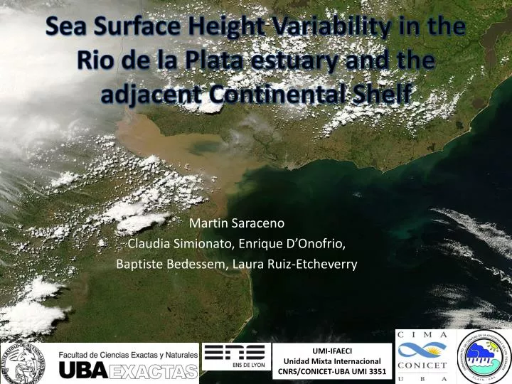
Sea Surface Height Variability in the Rio de la Plata estuary and the adjacent Continental Shelf. Martin Saraceno Claudia Simionato, Enrique D’Onofrio, Baptiste Bedessem, Laura Ruiz-Etcheverry. UMI-IFAECI Unidad Mixta Internacional CNRS/CONICET-UBA UMI 3351. Introduction: Rio de la Plata.

E N D
Sea Surface Height Variability in the Rio de la Plata estuary and the adjacent Continental Shelf Martin Saraceno Claudia Simionato, Enrique D’Onofrio, Baptiste Bedessem, Laura Ruiz-Etcheverry UMI-IFAECI Unidad Mixta Internacional CNRS/CONICET-UBA UMI 3351
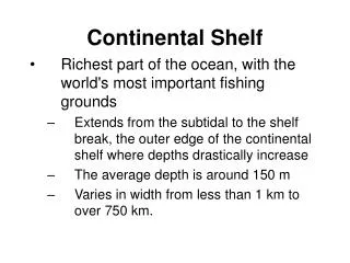
Introduction: Rio de la Plata • The Río de la Plata is the estuary formed by the confluence of the Uruguay River and the Paraná River on the border between Argentina and Uruguay. • Very populated region (Buenos Aires, Montevideo, + than 30million people) • Ecologically important: home of a large biodiveristy • - 290km long • one of the widest estuaries of the world: 220km maximum width • The Río de la Plata behaves as an estuary in which freshwater and seawater mix • Very shallow: upper part between 1 to 5m depth.
Introduction:: La Plata basin The position of the turbidity front corresponds to a submerged shoal “Barra del Indio” which acts as a barrier, dividing the Río de la Plata into an inner freshwater riverine area and an outer brackish estuarine area. The region is characterized by the discharge of the Rio de la Plata Sv (large variability discharge (22.000 m3/s, 8k a 80k). Imprtant storm surge events and upwelling events. Bla bla, ver introduccion articulos claudia
Introduction: Satellite altimetry in La Plata basin Large variability of Rio de la Plata has been well documented http://ctoh.legos.obs-mip.fr/
Can we use satellite SSH in the region to study spatio-temporal variability? Are altimetry corrections good enough? RMS Brazil-Malvinas Confluence: up to 40cm. RMS RdP: ~18cm. quite large. Real? Due to a physical process or is just bias because of not-so good corrections applied to the altimetry data? RMS (cm) of gridded SSH
Outline • Validation of along-track data with in-situ data • Analysis of spatio-temporal variability using gridded data
1. Comparison with in-situ data TG stations: Torre Oyarvide (hourly data, 1992-2009) & Spar-Brasileira (hourly data, 1 complete year) Closest distance between track 11 and Oyarvide: 22.8km Closest distance between track 102 and Spar-Brasileira: 11km Along track data used : CTOH, Jason 1 @ 1Hz and 20Hz, Jan. 2002-Jan. 2009 Uruguay Oyarvide Spar-Brasileira Argentina Track 102 Track 011 Background: RMS gridded SSH 1992-2011
1.a Comparison between data without corrections CTOH 20 Hz Oyarvide CTOH 1 Hz
1.a Comparison between data without corrections Spar-Brasileira Feb 2003- Feb 2004
1.b Evaluation of the correction terms • Two corrections are considered: • Tidal model • Atmospheric corrections (atmospheric pressure and wind effect) Tidal model CTOH offers 2 tidal model corrections: FES2004 and GOT47 In the Rio de la Plata and adjacent continental shelf region, both show good agreement with independent observations (Saraceno et al., CSR 2010). + enrique poster? Atmospheric correction This correction is crucial in this region: shallow bathymetry, complex coastline, coastal trapped waves propagation from the south contribute to amplify the SSH response to this correction term. CTOH uses the same correction used by AVISO: DAC (MOG2D, Carrère and Lyard, 2003). We compare MOG2D correction with in-situ low-pass (30hs) filtered data
1.b Evaluation of the correction terms DAC vs in-situ low-pass filtered data at Oyarvide Correlation: 0.86 (99%CL) RMSD: 22.8 cm R2=0.55 Comparison is not that good. A similar comparison in the North Atlantic shown that in coastal areas the validation against tide gauge data has shown that the largest improvement is achieved using HIPOCAS (HAMSOM, Hamburg regional model) and not DAC (Pascual et al., 2008). TO DO: use regional model with local bathymetry (already implemented using HAMSOM, Simionato et al., 2006) to check the atmospheric correction against DAC in the region.
2. Analysis of spatio-temporal variability using gridded data Along-track data available in the region Theoretical tracks Topex & Jason (red, 10 days), Envisat (yellow, 35 days), GFO (green, 17 days) When all satellite data are considered, spatial coverage is reasonable
EOF analysis of the seasonal component of the gridded SSH data • SSH in the region is dominated by seasonal variability. • We extracted the seasonal component by fitting to each grid point of the SSH the sum of an annual and semiannual wave. • We then estimate the EOF of the seasonal component First mode explains 78% of the seasonal signal Second mode First mode First mode
First mode + • Positive and negative phases of the first mode show two distinct pattern: • In the upper part of the estuary there no spatial variability. The estuary is very shallow and essentially behaves homogeneously; • In the lower part of the estuary and in the adjacent continental shelf there is a dipole-like spatial pattern. - How can we explain pattern 2? Let’s have a look to previous results obtained with other data..
a. Color images (SeaWiFS) + QuikSCAT winds + in-situ salinity Evidences of the time-space variability of the Plata plume, Piola et al., CSR 2008
2002-2010 seasonal average of chl-a from MODIS images using OC5 algorithm (IFREMER) Austral summer OC5 algorithm is designed to better separate chl-a from suspended organic particles Austral winter Simionato et al., in Press
b. Model outputs + Austral winter (JJA) SW Southwesterly winds produce a northward displacement of the buoyant plume. - Austral summer (JFM) NE Northeasterly winds produce a southwestwards retraction of the buoyant plume. In both cases, downwelling or upwelling can be generated as the result of Ekman transport. Ideal model simulation with constant SST. The result suggests that the SSH variability observed along the Uruguayan and Brazilian coast can have a component due to Ekman transport. Meccia et al., in press
Upwelling example SST SLA (m), CTOH 20Hz, track 178 SST along track 178 8-day averaged centered on 22 February 2008. 20-day upwelling favorable winds (Simionato et al., 2010).
Conclusions • - Comparison between along-track and in-situ data reveal that altimetry data correlates well in the region. However the implementation of a regional model for the atmospheric correction (pressure + wind) should be investigated. • First mode of the seasonal signal of gridded SSH satellite data suggests that is capturing the seasonal time-space variability of the Plata plume. • Upwelling events are captured by 20Hz along-track data
Perspectives (To do list): Better evaluate atmospheric corrections: Response of coastal sea level to wind is strongly dependent on the shelf width and on the shelf depth (it is quite clear from the motion equations). Hence, a model with a good shelf bathymetry will very likely give better results. We already have a regional model based on HAMSOM! (Simionato et a., 2006) Comparison of TG data to verify impact of the time-space variability of the Plata plume on SSH