Download
1 / 34
340 likes | 397 Vues
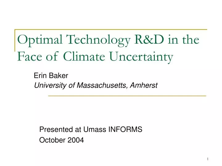
Optimal Technology R&D in the Face of Climate Uncertainty. Erin Baker University of Massachusetts, Amherst. Presented at Umass INFORMS October 2004. Today’s Talk. Background on Climate Change How to model R&D programs in top-down models? Theoretical results indicate that

E N D
Optimal Technology R&D in the Face of Climate Uncertainty Erin Baker University of Massachusetts, Amherst Presented at Umass INFORMS October 2004
Today’s Talk • Background on Climate Change • How to model R&D programs in top-down models? • Theoretical results indicate that • How R&D is modeled matters, and • How increasing risk is modeled matters. • Results and insights from numerical model. • Including uncertainty in the returns from R&D
Climate Change • Humans are changing the climate, through the accumulation of greenhouse gasses (GHG). • GHG are mainly emitted through the combustion of fossil fuels.
Human Contributions to the Greenhouse Effect Other CFCs 7% Methane 15% Carbon Dioxide 55% CFCs 11 and 12 17% Nitrous Oxide 6%
6 5 4 Natural Gas Billion Tons of Carbon 3 Oil Coal 2 1 0 1860 1885 1910 1935 1960 1985 Year Carbon Emissions Due to Fossil Fuel Consumption 1860 -1985
Climate Change • We have seen an increase of about 1°C over the last 100 years. • A doubling of CO2 from pre-industrial levels would increase global average temperatures by about 1.5 – 4.5°C • A 1.5°C rise would be warmest temperatures in last 6000 years. • A 4.5°C rise would raise temperatures to those last seen in time of dinosaurs.
Climate Change - Uncertainty • 100 years is a blip in geologic time. • Climate models are still in infancy. • Regional climate impacts are highly uncertain. • Human impacts of climate changes are uncertain. • Potential for catastrophic damages • Runaway greenhouse effect • Failure of the Gulf stream
Climate Change • Uncertainty about how emissions today will cause damages tomorrow. • But, we are learning more and more. • Uncertainty, learning, and adaptation impact current decisions • Conclusion: Uncertainty + Learning = less control of emissions. • Kolstad • Ulph & Ulph • Manne & Richels • Baker
What about R&D? • R&D planning is complicated by different programs • Solar PVs versus efficiency of coal-fired electricity • We consider optimal R&D • uncertainty and learning about climate damages • choice of R&D program
How to represent R&D? • Climate change is a complex problem, involving multiple variables. • In order to get insights about the best policy, we need a simple representation of alternative R&D programs. • What matters for climate change is how the technology that results from the R&D impacts the cost of abatement.
Climate Change Policy • We would like to choose a carbon emissions level that equated the marginal cost of abatement with the marginal damages from climate change. MC = MD • Technical change impacts the marginal cost of abatement.
t Q = f(t,e) e 0 e* The Production Function t = standard inputs e = emissions
t Q = f(t,e) e 0 e* From production function to abatement cost curve Production Function Abatement Cost Curve $ Cost a m 0 e = emissions m = emission reductions
Multiplicative Shift:Cost Reduction of No-Carbon Alternatives tmax Production Function Cost a a 1-a 1-a tmin m e e* 0 0 1 The abatement cost curve pivots downward
Emissions Reduction of Currently Economic Alternatives Production Function Cost a 1- a a 1- a a 1- a e m The abatement cost curve pivots to the right
Define Risk • How does optimal investment in R&D change with an increase in risk? • “Risk” – “uncertainty” – “Mean-preserving-spread” • See for example Rothschild & Stiglitz 1970,1971.
Theory Results • Proposition: Optimal R&D decreases with some increases in risk.
Theory Results • Proposition: Optimal R&D decreases with some increases in risk. • “Full abatement”
Theory Results • Proposition: Optimal R&D decreases with some increases in risk. • “Full abatement” • Fundamentally different from abatement result
Theory Results • The converse is not true – some R&D programs will always decrease in risk. • Individual R&D programs will react differently to an increase in risk. • It is crucial to model the specific program.
t t Cost Reduction Emissions reduction e e R&D impacts convexity of cost curve / production function Flatter R&D increases in risk More convex R&D decreases in risk
Integrated Assessment Model • William Nordhaus’s DICE • Optimal Growth + Climate Model • Social Planner chooses how to divide income between consumption, investment, and emissions reduction. • Added uncertainty, using stochastic programming. • First 5 periods decisions are made under uncertainty • After 5 periods the world splits into two damage scenarios.
Integrated Assessment Model • William Nordhaus’s DICE • Added R&D as a decision variable. • One time decision in 1st period before learning • Cost reduction implemented in 50 years, after learning about damages. • No uncertainty in the returns to R&D.
2 Types of increasing risk Increasing Probability certain low medium high Probability of high damage 0 .018 .05 .08333 Value of high damage - .042 .042 .042 Value of low damage .0035 .002794 .001473 0 Increasing Damage certain low medium high Probability of high damage 0 .018 .013 .002374 Value of high damage - .042 .057 .3 Value of low damage .0035 .002794 .002794 002794
1 1 0.9 0.1 3 0.78 1 1 0.75 0.75 0.82 0.25 0.25 0.33 0.33 3 3 0.18 0.33 4 Increasing Probability Increasing Damage Damage is on x-axis, Probability is on y-axis
1 1 0.9 0.1 3 0.78 1 1 0.75 0.67 0.82 0.33 0.25 0.33 0 3 3 0.18 0.33 4 Increasing Probability Increasing Damage Damage is on x-axis, Probability is on y-axis
1 1 0.9 0.1 3 0.78 1 1 0.75 0.67 0.86 0.33 0.25 0.33 0 3 3 0.14 0.33 5 Increasing Probability Increasing Damage Damage is on x-axis, Probability is on y-axis
16 0.4 12 0.3 8 Billions of US$ 0.2 Optimal R&D 4 0.1 0 0 0 0.02 0.04 0.06 0.08 0.1 0 0.02 0.04 0.06 0.08 0.1 Probability of high damage Probability of high damage Cost Reduction Emissions Reduction Results – Increasing Probability
0.16 5 4 0.12 3 Billions of US $ Optimal R&D 0.08 2 1 0.04 0 0 0 20 40 60 80 0 20 40 60 80 Cost Reduction Emissions Reduction % GDP Loss % GDP Loss Results – Increasing Damages
Conclusions • R&D can be a hedge against uncertainty. • But, it depends on what kind of R&D. • R&D into reducing the cost of low carbon alternatives • And what kind of risk. • Increasing the probability of needing very low carbon technologies, rather than considering higher levels of damages.
Unknowns • We need to estimate the relationship between investment in and R&D program, and the expected impact on the abatement cost curve. • We need to estimate the amount of uncertainty surrounding R&D programs.