Download
1 / 28
280 likes | 416 Vues
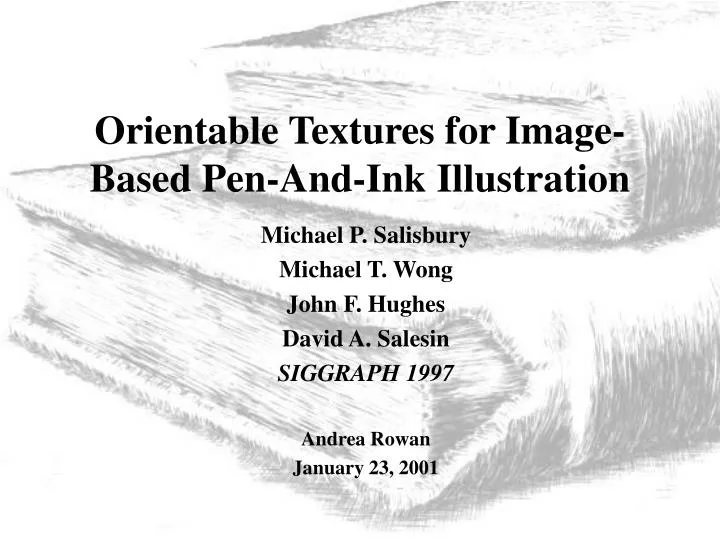
Orientable Textures for Image-Based Pen-And-Ink Illustration. Michael P. Salisbury Michael T. Wong John F. Hughes David A. Salesin SIGGRAPH 1997 Andrea Rowan January 23, 2001. Outline. Introduction to Image-Based Rendering Difference Image Algorithm Foundations Interactive System

E N D
Orientable Textures for Image-Based Pen-And-Ink Illustration Michael P. Salisbury Michael T. Wong John F. Hughes David A. Salesin SIGGRAPH 1997 Andrea Rowan January 23, 2001
Outline • Introduction to Image-Based Rendering • Difference Image Algorithm • Foundations • Interactive System • Rendering • Results • Problems • Future Work
Geometry-Based Systems Reads in 3-D geometry of scene Slow for complex objects Faster for walkthrough of scene / manipulation of objects Image-Based Systems Reads in a 2-D grayscale image Same speed for complex objects Slower for walkthrough of scene / manipulation of objects Introduction This paper’s algorithm uses an image- based system! vertices: 11159 faces: 13352 v -383.118 595.707 143.442 0.351793 0.169915 0.920527 v -376.05 577.648 143.533 0.294138 0.14277 0.94504 v -359.736 601.004 135.433 0.235886 0.183209 0.954354 v -404.41 671.841 143.49 0.757324 0.31507 0.572006 v -405.197 671.996 146.182 0.655538 -0.71832 0.232993 v -427.467 652.795 149.643 0.123845 -0.135311 0.983033 v -388.729 670.429 94.5347 0.537561 0.830288 0.147142
Algorithm - Foundations • Target (Tone) Image • Defines the tones at every point in the grayscale image • 0.0 (white) to 1.0 (black) 0.3 0.0 0.5 1.0 1.0 1.0
Algorithm - Foundations • Direction Field • Defines the desired orientation of strokes at each region of the illustration
Algorithm - Foundations • Stroke Example Set • Set of strokes that will be used to fill in tone areas • One stroke randomly chosen from the set each time
Interactive System • Editing tone - user can lighten or darken reference image
Interactive System • Editing direction - user can modify the direction image • comb - changes “direction” to match motion of cursor • blending tool - smooth between regions of different direction • region-filling tools Source tool Constant Direction Fill Interpolated Fill
Interactive System • Applying stroke • Vertical vector of stroke sample matches direction vector in direction image • Strokes placed dynamically (extra strokes for diverging field, strokes bent with direction) Direction image Static strokes Dynamic strokes
Rendering • Previous Steps were User-controlled • Rendering is entirely automated • importance - the fraction of darkness that has not been added to a section of the image. • Density of strokes is directly related to darkness in tone image.
Rendering - Steps • Making illustration match tone image • Illustration is b/w, and tone image is grayscale • Divide screen space into regions • Size of region depends on color in tone image (Larger regions for lighter areas of tone image) Regions Varying Region Size Constant Region Size
Rendering - Steps • Making illustration match tone image • When adding a stroke, add blurred stroke to region • Difference image = tone image value - blurred version of illustration value • Importance image = current difference value/initial difference value
Rendering - Steps Example: Consider a pixel with initial tone value of 0.2, initial illustration value (as for all regions) is 0. At the start: difference image = tone - blurred illustration = 0.2 - 0.0 = 0.2 importance image = current difference/initial difference = 0.2/0.2 = 1. Want this to approach zero or some min. threshold Add a stroke, which blurred, adds .15 to the value difference image = 0.2 - 0.15 = 0.05 importance image = .05/.2 = 0.025 Importance value decreases with each stroke.
Rendering - Steps • Drawing next Stroke in the Right Place • When a stroke is drawn, pixels in the area of the stroke lose their importance • Quadtree keeps track of most important pixel or region of pixels • Next stroke is drawn at most important pixel
Rendering - Steps • When to Stop the Illustration • Importance values get closer to zero with each stroke • Exact match of zero is difficult • Illustration stops when some minimum importance value is attained for each pixel
Rendering - Approximations • Assumption 1: Blurred version of multiple strokes is same as sum of blurred versions of independent strokes difference image = tone - blurred illustration OR difference image = tone - (blurred illustrationold + blurred strokenew) difference image = difference imageold - blurred strokenew
Rendering - Approximations • Assumption 1: Cont’d • Depends on strokes not overlapping • Points where strokes cross will be counted as darkened twice • Illustration is in black & white, so two strokes crossed is the same darkness as one stroke • Solution is hacked with lightening factor stored in a “darkness-look-up-table” • Example: • If region is 50% gray (0.5), 90% of pixels drawn are visible • Reduce darkness of blurred strokes to 90% before adding blurred value to illustration
Rendering - Approximations • Assumption 2: Simplified filtered image of stroke for computations • Render control hull as blurry line • Width = 2h/t • h = stroke thickness (mm) • t = desired tone value (0.0=white to 1.0=black) • Clamped from 1 to 10 mm.
Drawing a Stroke • Orienting and Bending • Control hull - frame around each stroke • Broken into parts and mapped to direction image Stroke Direction image Illustration Pi+3 Pi+3 Pi+2 Pi+2 Pi+1 Pi+1 Pi Pi
Drawing a Stroke • Clipping • When direction field changes rapidly • When stroke crosses into a region that is already dark enough
Output Enhancements • Variable Width • Pen and ink pressure can vary from start of stroke to end • Each stroke has 3 widths • Start width • Middle width • End width • Different ratios if drawing hair vs. shadows
Output Enhancements • “Wiggles” • Artists don’t draw with rulers! • For strokes > 5 mm • Add control points to control hull • Random perturbation within range (-0.15 to 0.15 mm)
Results • Stroke density adjusts for different sized images
Results Performance (SGI 180MHz R500 processor)
Other Work • Michael Kowalski et al., “Art-Based Rendering of Fur, Grass, and Trees,” SIGGRAPH 1999 • Use off-screen grayscale rendering of scene as reference image • Convert 2-D screen position to 3-D space for interactive geometry-based system
Accomplishments • Textures appear attached to objects (this is difficult in image-based rendering) • Good algorithm for stroke density in image-based rendering
Problems • High degree of user-tweaking (direction image) • Direct user interaction with illustration causes performance hit • Poor performance (every pixel is looked at)
Future Work • User interaction with pen-and-ink illustration, not direction image • Support of coherent textures (bricks, fabrics, etc.)