Download
1 / 26
260 likes | 330 Vues
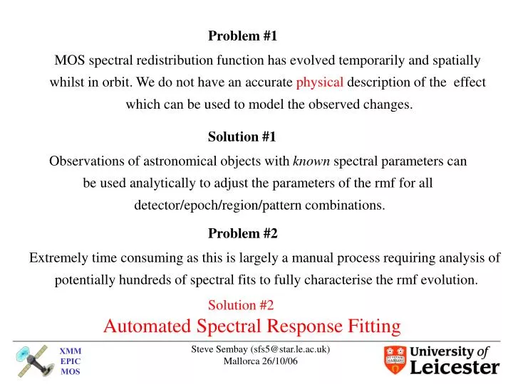
Problem #1. MOS spectral redistribution function has evolved temporarily and spatially whilst in orbit. We do not have an accurate physical description of the effect which can be used to model the observed changes. Solution #1.

E N D
Problem #1 MOS spectral redistribution function has evolved temporarily and spatially whilst in orbit. We do not have an accurate physical description of the effect which can be used to model the observed changes. Solution #1 Observations of astronomical objects with known spectral parameters can be used analytically to adjust the parameters of the rmf for all detector/epoch/region/pattern combinations. Problem #2 Extremely time consuming as this is largely a manual process requiring analysis of potentially hundreds of spectral fits to fully characterise the rmf evolution. Solution #2 Automated Spectral Response Fitting
σnew(1.49) = p x σold(1.49) E = 1.49 keV model ga σ = 0.0 N = free Code development by Jenny function myfunct, p ; p(n) newccf = rmf_param_adjust(p, oldccf) rmf = rmfgen(newccf) chisq = xspec_fit(spectrum, model, rmf) return, chisq end pro rmfmin, p, chimin result = tnmin(‘myfunct’, p, bestmin=chimin, /autoderivative) newccf = rmf_param_adjust(result, oldccf) return end
;+ ; NAME: ; TNMIN ; ; AUTHOR: ; Craig B. Markwardt, NASA/GSFC Code 662, Greenbelt, MD 20770 ; craigm@lheamail.gsfc.nasa.gov ; UPDATED VERSIONs can be found on my WEB PAGE: ; http://cow.physics.wisc.edu/~craigm/idl/idl.html ; ; PURPOSE: ; Performs function minimization (Truncated-Newton Method) ; ; MAJOR TOPICS: ; Optimization and Minimization ; ; CALLING SEQUENCE: ; parms = TNMIN(MYFUNCT, X, FUNCTARGS=fcnargs, NFEV=nfev, ; MAXITER=maxiter, ERRMSG=errmsg, NPRINT=nprint, ; QUIET=quiet, XTOL=xtol, STATUS=status, ; FGUESS=fguess, PARINFO=parinfo, BESTMIN=bestmin, ; ITERPROC=iterproc, ITERARGS=iterargs, niter=niter) ; ; DESCRIPTION: ; ; TNMIN uses the Truncated-Newton method to minimize an arbitrary IDL ; function with respect to a given set of free parameters. Blah…….
function myfunct, p ; p(n) newccf = rmf_param_adjust(p, oldccf) rmf = rmfgen(newccf) chisq = xspec_fit(spectrum, model, rmf) return, chisq end Slow ~ secs to mins pro rmfmin, p, chimin result = tnmin(‘myfunct’, p, bestmin=chimin, /autoderivative) newccf = rmf_param_adjust(result, oldccf) return end
Results from 3 sets of tests: Fitting the Al calibration line(s) at epoch Rev 110-169 Fitting the low energy continuum of 3C273 at epoch 0-109 Fitting the continuum of RXJ1856 at epoch 744+ Mono-pixel spectra used throughout
“Red” wing is due to incomplete charge collection rather than intrinsic broadening Al Kα = Kα1(1.4867) + 0.5 x Kα2(1.4863) In our analytic rmf model we model this by splitting the profile “Red” side = Gaussian(σ) + Gaussian(R x σ) “Blue” side = Gaussian(σ) Normalisations match at join Test #1: Resolution at Al Kα In our automatic fitting we adjust the values of σ (~30) and R (~1.5) at 1.487 keV by “fudge” factors, p, such that σnew = p1 x σold Rnew = p2 x Rold
Spectral Model: (ga + ga + ga) Fit Range: 1.4-1.56 keV Proc. Time = 1.72 hrs P1 = 1.047 P2 = 0.894 Χ2ν = 7.74 P1 = 1.0 P2 = 1.0 Χ2ν = 18.4 Test #1: Resolution at Al Kα β1 E = 1.5574, σ = 0.0, N = 0.01N0 α2 E = 1.4863, σ = 0.0, N = 0.5N0 α1 E = 1.4867, σ = 0.0, N0 = free
Test #1: Resolution at Al Kα MOS1 Mg XI line in Zeta Puppis, Rev 0156, RGS Model
Energy Epoch Test #2: Low energy continuum of 3C 273 (Rev 0094) Continuum (“hard power law + soft excess”) fits to 3c 273 TU Mode TU Mode MOS1 ratio image
1.0 f(d) f(d) = α + βd d < d0 = 1.0 d ≥ d0 α 0.0 d0 d β α Test #2: Low energy continuum of 3C 273 (Rev 0094) Surface Loss Function Eobs(d) = Ein(d) x f(d) Integrate over d to get profile
Fudge factor defined at 350, 500, 650 eV Test #2: Low energy continuum of 3C 273 (Rev 0094) Alpha Parameter v Energy, Epoch Rev 0-109
Spectral Model: phabs * (po + po) Fit Range: 0.1-1.0 keV Rev 0094 Proc. Time: 3.9 Hrs Χ2ν = 3.01 Χ2ν = 1.97 Test #2: Low energy continuum of 3C 273 (Rev 0094) Γ = 1.644, N0 = 0.0194 Γ = Free, N0 = Free nH = 1.79 x 1020 cm-2
Test #2: Low energy continuum of 3C 273 (Rev 0094) Alpha Parameter v Energy, Epoch Rev 0-109 Fudge factor defined at 350, 500, 650 eV
Test #2: Low energy continuum of 3C 273 (Rev 0094) Fit model to PN and fold through MOS1 (old and new rmf)
Test #2: Low energy continuum of 3C 273 (Rev 0094) RGS model (renormalised) fit to MOS1 in 0.1-0.55 keV band
Test #3: BB fits to RXJ1856 (Rev 0798) MOS1 Core nH = 1.4(0.1)E20 kT = 61.4(0.2) eV MOS1 Wings nH = 1.1(0.2)E20 kT = 60.3(0.4) eV
Test #3: BB fits to RXJ1856 (Rev 0798) MOS2 Core nH = 0.93(0.1)E20 kT = 62.0(0.3) eV MOS2 Wings nH = 0.98(0.2)E20 kT = 59.7(0.5) eV
Spectral Model: phabs * bb Fit Range: 0.1-1.0 keV Test #3: BB fits to RXJ1856 (Rev 0798) kT = 62 eV, N0 = Free nH = 0.75 x 1020 cm-2 Parameters reported by Vadim/Frank for pn at previous Cal. meeting Fudge Factors: alpha surface loss parameters at…..250, 350, 450, 550 eV
Test #3: BB fits to RXJ1856 (Rev 0798) Fit to MOS1 data with new rmf
Test #3: BB fits to RXJ1856 (Rev 0798) Fit to MOS2 data with new rmf
Test #3: BB fits to RXJ1856 (Rev 0798) Fit to MOS1 3c 273 data with old/new rmf nH = 2.6(0.2)e20 cm-2 nH = 2.1(0.2)e20 cm-2
Test #3: BB fits to RXJ1856 (Rev 0798) Fit to MOS2 3c 273 data with old/new rmf nH = 2.4(0.2)e20 cm-2 nH = 1.9(0.2)e20 cm-2
Conclusions • Algorithm works! • Timely results can be gained even using a single CPU, but we intend to port code to the multi(250) processor central computing facility at Leicester • Smoothing out the residuals in early MOS 3c 273 data improves cross-calibration with pn and probably rgs • Forcing spectral agreement between MOS and pn in RXJ1856 improves residuals in contemporary MOS2 3c 273 data