Download
1 / 26
270 likes | 564 Vues
Random slope. Varying slopes . Basic Model:. Varying slopes. Gelman and Hill Presentation. Varying slopes. The really tricky part is that correlation term—higher group level errors in the DV may also be connected to higher (or lower) effects of X. . In R it is pretty easy.

E N D
Varying slopes • Basic Model:
Varying slopes • Gelman and Hill Presentation
Varying slopes • The really tricky part is that correlation term—higher group level errors in the DV may also be connected to higher (or lower) effects of X.
In R it is pretty easy • Just add which individual level effect you want to vary as a function of the group • Two examples • Radon • NES • Add the second random term by putting the variable before the |”group” • Add second level predictors in the random slope by creating an interaction
R output Linear mixed-effects model fit by REML Formula: y ~ x + u.full + x:u.full + (1 + x | county) AIC BIC logLik MLdeviance REMLdeviance 2141 2174 -1063 2114 2127 Random effects: Groups Name Variance Std.Dev. Corr county (Intercept) 0.0155 0.124 x 0.0942 0.307 0.409 Residual 0.5617 0.749 number of obs: 919, groups: county, 85 • Random effects who the varainces and the correlation
Output Fixed effects: Estimate Std. Error t value (Intercept) 1.4686 0.0352 41.7 x -0.6710 0.0844 -7.9 u.full 0.8081 0.0906 8.9 x:u.full -0.4195 0.2271 -1.8 Correlation of Fixed Effects: (Intr) x u.full x -0.241 u.full 0.208 -0.093 x:u.full -0.093 0.173 -0.231 • The fixed effects coefficients are the gamma terms
NES output Linear mixed-effects model fit by REML Formula: y ~ x + u.full + x:u.full + (1 + x | district) AIC BIC logLik MLdeviance REMLdeviance 11720 11756 -5853 11722 11706 Random effects: Groups Name Variance Std.Dev. Corr district (Intercept) 92.6 9.62 x 201.1 14.18 -0.542 Residual 951.4 30.85 number of obs: 1199, groups: district, 139
NES Output Fixed effects: Estimate Std. Error t value (Intercept) 43.97 2.81 15.62 x 10.44 3.57 2.93 u.full 3.61 4.24 0.85 x:u.full 4.70 5.33 0.88 Correlation of Fixed Effects: (Intr) x u.full x -0.764 u.full -0.664 0.507 x:u.full 0.512 -0.669 -0.769
What do these mean? • Effects of race depends on whether or not Bush carried the county.
Wishart • What if we have 2 or more X’s?
Problem? • Each level one independent variable adds one variance parameter and k covariance parameters • Change notation to matrix form: • X is an NxK+1 matrix of level one predictors • β is the JxK+1 matrix of the coefficients • Zj is the JxL (L is the number of Z’s) matrix of predictors
Problem • Γ is the LxK matrix of coefficients for the group level predictors • Τ is the variance covariance matrix for the group level errors • Note: Adding x’s whose effect does not vary is not a complication.
Problem • So, I said there was a problem here and there is. It is the Τ matrix. • What is this? Again, it is the variance-covariance matrix of the second level errors • So? These matrices (var-cov) have some properties. • It must be positive definite. • Estimates of each element place limits on the other parts • Think of it as a correlation matrix
Solution? • Inverse Wishart • This is a multivariate distribution • Defines the pdf of a matrix • Τ~Inv-WishartK+1(I) • It is the multivariate generalization of the Inverse Gamma • I know that is not all that helpful. • The inverse gamma is continuous, non-monotonic, based on two parameters, and strictly positive
Back to the Inverse Wishart • Two parameters • Degrees of freedom (K+1) • Scale (I) • Setting the df and scale to those means: • Df sets the correlations in the errors to a uniform (-1,1) distribution (that’s nice) • This constrains the variances and covariances. That’s bad we want to estimate them.
Wishart • If we change the df, we can estimate the variances and covariances. Add a scale parameterξk (xi) • Variances are the diagonals of the unscaled matrix Q multiplied by a scaling factor:
Covariances are similar: • We don’t care about the parameters in the Inverse Wishart. They have no inherent meaning, nor are they theoretically interesting. • They are useful in making sure the variance/covariance matrix (and the correlation matrix) are nicely behaved.
There is a logic to this we will use later • We have a problem with the estimates • The parameters constrain each other • Hard to separate them • Rather than make a series of modeling choices (each is from a normal and let’s estimate them independently), let’s make one big modeling choice and solve all the problems • This is not an “assumption” about the errors. • They are still normal.
So, what are these correlations? • How the variance in the parameter estimates connect—does a higher than average constant occur with muted or heightened effects of the X variable? • Not usually all that interesting—something of a nuisance parameter.