Download
1 / 150
1.51k likes | 1.71k Vues
ECE/CS 757: Advanced Computer Architecture II. Instructor:Mikko H Lipasti Spring 2013 University of Wisconsin-Madison

E N D
ECE/CS 757: Advanced Computer Architecture II Instructor:Mikko H Lipasti Spring 2013 University of Wisconsin-Madison Lecture notes based on slides created by John Shen, Mark Hill, David Wood, GuriSohi, Jim Smith, Natalie Enright Jerger, Michel Dubois, MuraliAnnavaram, Per Stenström and probably others
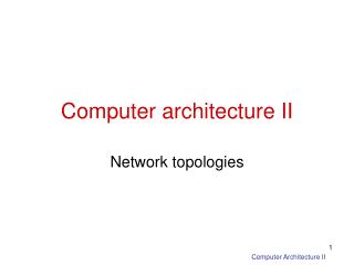
Lecture Outline • Introduction to Networks • Network Topologies • Network Routing • Network Flow Control • Router Microarchitecture • Technology example: On-chip Nanophotonics Mikko Lipasti-University of Wisconsin
Introduction • How to connect individual devices into a group of communicating devices? • A device can be: • Component within a chip • Component within a computer • Computer • System of computers • Network consists of: • End point devices with interface to network • Links • Interconnect hardware • Goal: transfer maximum amount of information with the least cost (minimum time, power) Mikko Lipasti-University of Wisconsin
Types of Interconnection Networks • Interconnection networks can be grouped into four domains • Depending on number and proximity of devices to be connected • On-Chip networks (OCNs or NoCs) • Devices include microarchitectural elements (functional units, register files), caches, directories, processors • Current designs: small number of devices • Ex: IBM Cell, Sun’s Niagara • Projected systems: dozens, hundreds of devices • Ex: Intel Teraflops research prototypes, 80 cores • Proximity: millimeters Mikko Lipasti-University of Wisconsin
Types of Interconnection Networks (2) • System/Storage Area Network (SANs) • Multiprocessor and multicomputer systems • Interprocessor and processor-memory interconnections • Server and data center environments • Storage and I/O components • Hundreds to thousands of devices interconnected • IBM Blue Gene/L supercomputer (64K nodes, each with 2 processors) • Maximum interconnect distance typically on the order of tens of meters, but some with as high as a few hundred meters • InfiniBand: 120 Gbps over a distance of 300 m • Examples (standards and proprietary) • InfiniBand, Myrinet, Quadrics, Advanced Switching Interconnect Mikko Lipasti-University of Wisconsin
Types of Interconnection Networks (3) • Local Area Network (LANs) • Interconnect autonomous computer systems • Machine room or throughout a building or campus • Hundreds of devices interconnected (1,000s with bridging) • Maximum interconnect distance on the order of few kilometers, but some with distance spans of a few tens of kilometers • Example (most popular): 1-10Gbit Ethernet Mikko Lipasti-University of Wisconsin
Types of Interconnection Networks (4) • Wide Area Networks (WANs) • Interconnect systems distributed across the globe • Internetworking support is required • Many millions of devices interconnected • Maximum interconnect distance of many thousands of kilometers • Example: ATM Mikko Lipasti-University of Wisconsin
Organization • Here we focus on On-chip networks • Concepts applicable to all types of networks • Focus on trade-offs and constraints as applicable to NoCs Mikko Lipasti-University of Wisconsin
On-Chip Networks (NoCs) • Why Network on Chip? • Ad-hoc wiring does not scale beyond a small number of cores • Prohibitive area • Long latency • OCN offers • scalability • efficient multiplexing of communication • often modular in nature (ease verification) Mikko Lipasti-University of Wisconsin
Differences between on-chip and off-chip networks • Off-chip: I/O bottlenecks • Pin-limited bandwidth • Inherent overheads of off-chip I/O transmission • On-chip • Tight area and power budgets • Ultra-low on-chip latencies Mikko Lipasti-University of Wisconsin
MulticoreExamples (1) 0 1 2 3 4 5 0 1 XBAR 2 3 4 5 Sun Niagara Mikko Lipasti-University of Wisconsin
MulticoreExamples (2) • Element Interconnect Bus • 4 rings • Packet size: 16B-128B • Credit-based flow control • Up to 64 outstanding requests • Latency: 1 cycle/hop RING IBM Cell Mikko Lipasti-University of Wisconsin
Many Core Example • Intel Polaris • 80 core prototype • Academic Research ex: • MIT Raw, TRIPs • 2-D Mesh Topology • Scalar Operand Networks 2D MESH Mikko Lipasti-University of Wisconsin
References • William Dally and Brian Towles. Principles and Practices of Interconnection Net- works. Morgan Kaufmann Pub., San Francisco, CA, 2003. • William Dally and Brian Towles, “Route packets not wires: On-chip interconnection networks,” in Proceedings of the 38th Annual Design Automation Conference (DAC-38), 2001, pp. 684–689. • David Wentzlaff, Patrick Griffin, Henry Hoffman, LieweiBao, Bruce Edwards, Carl Ramey, Matthew Mattina, Chi-Chang Miao, John Brown I I I, and AnantAgarwal. On-chip interconnection architecture of the tile processor. IEEE Micro, pages 15– 31, 2007. • Michael Bedford Taylor, Walter Lee, SamanAmarasinghe, and AnantAgarwal. Scalar operand networks: On-chip interconnect for ILP in partitioned architectures. In Proceedings of the International Symposium on High Performance Computer Architecture, February 2003. • S. Vangal, J. Howard, G. Ruhl, S. Dighe, H. Wilson, J. Tschanz, D. Finan, P. Iyer, A. Singh, T. Jacob, S. Jain, S. Venkataraman, Y. Hoskote, and N. Borkar. An 80-tile 1.28tflops network-on-chip in 65nm cmos. Solid-State Circuits Conference, 2007. ISSCC 2007. Digest of Technical Papers. IEEE International, pages 98–589, Feb. 2007. Mikko Lipasti-University of Wisconsin
Lecture Outline • Introduction to Networks • Network Topologies • Network Routing • Network Flow Control • Router Microarchitecture • Technology example: On-chip Nanophotonics Mikko Lipasti-University of Wisconsin
Topology Overview • Definition: determines arrangement of channels and nodes in network • Analogous to road map • Often first step in network design • Routing and flow control build on properties of topology Mikko Lipasti-University of Wisconsin
Abstract Metrics • Use metrics to evaluate performance and cost of topology • Also influenced by routing/flow control • At this stage • Assume ideal routing (perfect load balancing) • Assume ideal flow control (no idle cycles on any channel) • Switch Degree: number of links at a node • Proxy for estimating cost • Higher degree requires more links and port counts at each router Mikko Lipasti-University of Wisconsin
Latency • Time for packet to traverse network • Start: head arrives at input port • End: tail departs output port • Latency = Head latency + serialization latency • Serialization latency: time for packet with Length L to cross channel with bandwidth b (L/b) • Hop Count: the number of links traversed between source and destination • Proxy for network latency • Per hop latency with zero load Mikko Lipasti-University of Wisconsin
Impact of Topology on Latency • Impacts average minimum hop count • Impact average distance between routers • Bandwidth Mikko Lipasti-University of Wisconsin
Throughput • Data rate (bits/sec) that the network accepts per input port • Max throughput occurs when one channel saturates • Network cannot accept any more traffic • Channel Load • Amount of traffic through channel c if each input node injects 1 packet in the network Mikko Lipasti-University of Wisconsin
Maximum channel load • Channel with largest fraction of traffic • Max throughput for network occurs when channel saturates • Bottleneck channel Mikko Lipasti-University of Wisconsin
Bisection Bandwidth • Cuts partition all the nodes into two disjoint sets • Bandwidth of a cut • Bisection • A cut which divides all nodes into nearly half • Channel bisection min. channel count over all bisections • Bisection bandwidth min. bandwidth over all bisections • With uniform traffic • ½ of traffic cross bisection Mikko Lipasti-University of Wisconsin
Throughput Example • Bisection = 4 (2 in each direction) 0 1 2 3 4 5 6 7 • With uniform random traffic • 3 sends 1/8 of its traffic to 4,5,6 • 3 sends 1/16 of its traffic to 7 (2 possible shortest paths) • 2 sends 1/8 of its traffic to 4,5 • Etc • Channel load = 1 Mikko Lipasti-University of Wisconsin
Path Diversity • Multiple minimum length paths between source and destination pair • Fault tolerance • Better load balancing in network • Routing algorithm should be able to exploit path diversity • We’ll see shortly • Butterfly has no path diversity • Torus can exploit path diversity Mikko Lipasti-University of Wisconsin
Path Diversity (2) • Edge disjoint paths: no links in common • Node disjoint paths: no nodes in common except source and destination • If j = minimum number of edge/node disjoint paths between any source-destination pair • Network can tolerate j link/node failures • Path diversity does not provide pt-to-pt order • Implications on coherence protocol design! Mikko Lipasti-University of Wisconsin
Symmetry • Vertex symmetric: • An automorphism exists that maps any node a onto another node b • Topology same from point of view of all nodes • Edge symmetric: • An automorphism exists that maps any channel a onto another channel b Mikko Lipasti-University of Wisconsin
Direct & Indirect Networks • Direct: Every switch also network end point • Ex: Torus • Indirect: Not all switches are end points • Ex: Butterfly Mikko Lipasti-University of Wisconsin
Torus (1) • K-ary n-cube: knnetwork nodes • n-dimensional grid with k nodes in each dimension 3-ary 2-cube 3-ary 2-mesh 2,3,4-ary 3-mesh Mikko Lipasti-University of Wisconsin
Torus (2) • Topologies in Torus Family • Ring k-ary 1-cube • Hypercubes 2-ary n-cube • Edge Symmetric • Good for load balancing • Removing wrap-around links for mesh loses edge symmetry • More traffic concentrated on center channels • Good path diversity • Exploit locality for near-neighbor traffic Mikko Lipasti-University of Wisconsin
Torus (3) • Hop Count: • Degree = 2n, 2 channels per dimension Mikko Lipasti-University of Wisconsin
Channel Load for Torus • Even number of k-ary (n-1)-cubes in outer dimension • Dividing these k-ary (n-1)-cubes gives 2 sets of kn-1 bidirectional channels or 4kn-1 • ½ Traffic from each node cross bisection • Mesh has ½ the bisection bandwidth of torus Mikko Lipasti-University of Wisconsin
Torus Path Diversity 2 dimensions* NW, NE, SW, SE combos 2 edge and node disjoint minimum paths n dimensions with Δi hops in i dimension *assume single direction for x and y Mikko Lipasti-University of Wisconsin
Implementation • Folding • Equalize path lengths • Reduces max link length • Increases length of other links 0 1 2 3 3 2 1 0 Mikko Lipasti-University of Wisconsin
Concentration • Don’t need 1:1 ratio of network nodes and cores/memory • Ex: 4 cores concentrated to 1 router Mikko Lipasti-University of Wisconsin
Butterfly • K-ary n-fly: knnetwork nodes • Example: 2-ary 3-fly • Routing from 000 to 010 • Dest address used to directly route packet • Bit n used to select output port at stage n 0 1 0 0 0 00 10 20 1 1 2 2 01 11 21 3 3 4 4 02 12 22 5 5 6 6 03 13 23 7 7 Mikko Lipasti-University of Wisconsin
Butterfly (2) • No path diversity • Hop Count • Logkn + 1 • Does not exploit locality • Hop count same regardless of location • Switch Degree = 2k • Channel Load uniform traffic • Increases for adversarial traffic Mikko Lipasti-University of Wisconsin
Flattened Butterfly • Proposed by Kim et al (ISCA 2007) • Adapted for on-chip (MICRO 2007) • Advantages • Max distance between nodes = 2 hops • Lower latency and improved throughput compared to mesh • Disadvantages • Requires higher port count on switches (than mesh, torus) • Long global wires • Need non-minimal routing to balance load Mikko Lipasti-University of Wisconsin
Flattened Butterfly • Path diversity through non-minimal routes Mikko Lipasti-University of Wisconsin
Clos Network rxr input switch nxm input switch mxn output switch rxr input switch nxm input switch mxn output switch rxr input switch nxm input switch mxn output switch rxr input switch nxm input switch mxn output switch rxr input switch Mikko Lipasti-University of Wisconsin
Clos Network • 3-stage indirect network • Characterized by triple (m, n, r) • M: # of middle stage switches • N: # of input/output ports on input/output switches • R: # of input/output switching • Hop Count = 4 Mikko Lipasti-University of Wisconsin
Folded Clos (Fat Tree) • Bandwidth remains constant at each level • Regular Tree: Bandwidth decreases closer to root Mikko Lipasti-University of Wisconsin
Fat Tree (2) • Provides path diversity Mikko Lipasti-University of Wisconsin
Common On-Chip Topologies • Torus family: mesh, concentrated mesh, ring • Extending to 3D stacked architectures • Favored for low port count switches • Butterfly family: Flattened butterfly Mikko Lipasti-University of Wisconsin
Topology Summary • First network design decision • Critical impact on network latency and throughput • Hop count provides first order approximation of message latency • Bottleneck channels determine saturation throughput Mikko Lipasti-University of Wisconsin
Lecture Outline • Introduction to Networks • Network Topologies • Network Routing • Network Flow Control • Router Microarchitecture • Technology example: On-chip Nanophotonics Mikko Lipasti-University of Wisconsin
Routing Overview • Discussion of topologies assumed ideal routing • Practically though routing algorithms are not ideal • Discuss various classes of routing algorithms • Deterministic, Oblivious, Adaptive • Various implementation issues • Deadlock Mikko Lipasti-University of Wisconsin
Routing Basics • Once topology is fixed • Routing algorithm determines path(s) from source to destination Mikko Lipasti-University of Wisconsin
Routing Algorithm Attributes • Number of destinations • Unicast, Multicast, Broadcast? • Adaptivity • Oblivious or Adaptive? Local or Global knowledge? • Implementation • Source or node routing? • Table or circuit? Mikko Lipasti-University of Wisconsin
Oblivious • Routing decisions are made without regard to network state • Keeps algorithms simple • Unable to adapt • Deterministic algorithms are a subset of oblivious Mikko Lipasti-University of Wisconsin
Deterministic • All messages from Src to Dest will traverse the same path • Common example: Dimension Order Routing (DOR) • Message traverses network dimension by dimension • Aka XY routing • Cons: • Eliminates any path diversity provided by topology • Poor load balancing • Pros: • Simple and inexpensive to implement • Deadlock free Mikko Lipasti-University of Wisconsin