Download
1 / 8

E N D
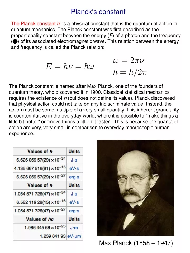
Planck’s constant The Planck constant h is a physical constant that is the quantum of action in quantum mechanics. The Planck constant was first described as the proportionality constant between the energy (E) of a photon and the frequency (n) of its associated electromagnetic wave. This relation between the energy and frequency is called the Planck relation: The Planck constant is named after Max Planck, one of the founders of quantum theory, who discovered it in 1900. Classical statistical mechanics requires the existence of h (but does not define its value). Planck discovered that physical action could not take on any indiscriminate value. Instead, the action must be some multiple of a very small quantity. This inherent granularity is counterintuitive in the everyday world, where it is possible to "make things a little bit hotter" or "move things a little bit faster". This is because the quanta of action are very, very small in comparison to everyday macroscopic human experience. Max Planck (1858 – 1947)
The Einstein Model of a Solid In 1907, Einstein proposed a model that reasonably predicted the thermal behavior of crystalline solids (a 3D bed-spring model): A crystalline solid containing N atoms behaves as if it contained 3Nidenticalindependent quantum harmonic oscillators, each of which can store an integer number ni of energy units = ħ. We can treat a 3D harmonic oscillator as if it were oscillating independently in 1D along each of the three axes. classic oscillator: quantum oscillator: principal h.o. quantum number 1D harmonic oscillator
ħ 1 3 2 3N the solid’s internal energy (assume N atoms; 3N oscillators) the zero-point energy (subtracted) all oscillators are identical, the energy quanta are the same The conceptual Einstein solid is useful for examining the idea of multiplicity in the distribution of energy among the available energy states of the system. All of the energy levels are considered to be equally probable within the constraint of having q units of energy and 3N oscillators. At high T ≫ħ (the classical limit of large ni): To describe a macrostate of an Einstein solid, we have to specify N and U, a microstate ni for 3N oscillators.
Example: the “macrostates” of an Einstein Model with only one atom
Another example: q=3 units of energy distributed in an Einstein solid with N=4 oscillators. At left is the detailed listing of the possible distributions of the energy, a total of 20 different distributions for 3 units of energy among 4 oscillators (a multiplicity of 20). If we are trying to develop a description of a real solid with Avogadro's number of oscillators, this kind of approach is clearly impractical. Fortunately, mathematical expressions for the multiplicity make the task manageable. distributing q pebbles over N boxes distributing q pebbles over N-1 partitions q dots and N-1 lines for a total of q+N-1 symbols! The multiplicity of a state of N oscillators (N/3 atoms) with q energy quanta distributed among these oscillators: For the example above :
Interacting systems. Two Einstein Solids. To understand irreversible processes and the second law, we now move on to consider a system of two Einstein solids, A and B, which are free to exchange energy with each other but isolated from the rest of the universe. First we should be clear about what is meant by the “macrostate” of such a composite system. For simplicity, we assume that our two solids are weakly coupled, so that the exchange of energy between them is much slower than the exchange of energy among atoms within each solid. Then the individual energies of the two solids, UAand UB, will change only slowly; over sufficiently short time scales they are essentially fixed. We will use the word “macrostate” to refer to the state of the combined system, as specified by the (temporarily) constrained values of UAand UB. For any such macrostate we can compute the multiplicity. However, on longer time scales the values of UA and UBwill change, so we will also talk about the total multiplicity of the combined system, considering all microstates to be “accessible” with only Utotal = UA + UBheld fixed. In any case, we must also specify the number of oscillators in each solid, NA and NB, in order to fully describe the macrostate of the system. Let us start with a very small system, in which each of the “solids” contains only three oscillators and the solids share a total of six units of energy: There are seven possible macrostates, with qA = 0, 1, . . . 6. For each of these macrostates, we can compute the multiplicity of the combined system as the product of the multiplicities of the individual systems:
From the table we see that the fourth macrostate, in which each solid has three units of energy, has the highest multiplicity (100). Now let us invoke the fundamental assumption: On long time scales, all of the 462 microstates are accessible to the system, and therefore, by assumption, are equally probable. The probability of finding the system in any given macrostate is therefore proportional to that macrostate’s multiplicity. For instance, in this example the fourth macrostate is the most probable, and we would expect to find the system in this macrostate 100/462 of the time. The macrostates in which one solid or the other has all six units of energy are less probable, but not overwhelmingly so. All microstates are equally probable, but some macrostates are more probable than others! We see immediately that the multiplicities are now quite large. But more importantly, the multiplicities of the various macrostates now differ by factors that can be very large - more than 1033 in the most extreme case. If we again make the fundamental assumption, this result implies that the most likely macrostates are 1033 times more probable than the least likely macrostates. If this system is initially in one of the less probable macrostates, and we then put the two solids in thermal contact and wait a while, we are almost certain to find it fairly near the most probable macrostate of qA = 60 when we check again later. In other words, this system will exhibit irreversible behavior, with net energy flowing spontaneously from one solid to the other, until it is near the most likely macrostate. This conclusion is just a statement of the second law of thermodynamics.
Using this result, we can state the second law more strongly: Aside from fluctuations that are normally much too small to measure, any isolated macroscopic system will inevitably evolve toward its most likely accessible macrostate. Although we have proved this result only for a system of two weakly coupled Einstein solids, similar results apply to all other macroscopic systems. The details of the counting become more complex when the energy units can come in different sizes, but the essential properties of the combinatorics of large numbers do not depend on these details. If the subsystems are not weakly coupled, the division of the whole system into subsystems becomes a mere mental exercise with no real physical basis; nevertheless, the same counting arguments apply, and the system will still exhibit irreversible behavior if it is initially in a macrostate that is in some way “inhomogeneous”. We observe that energy flows spontaneously from one block (A) to the other (B). We say that block A has a higher temperature than block B. In fact, we say that the energy flow occurs because the blocks have different temperatures. We further observe that after the lapse of some time, called the relaxation time, the flow of energy from A to B ceases, after which there is zero net transfer of energy between the blocks. At this point the two blocks are in thermal equilibrium with each other, and we would say that they have the same temperature. Heat is a probabilistic phenomenon, not absolutely certain, but extremely likely. The spontaneous flow of energy stops when a system is at, or very near, its most likely macrostate (i.e., the one with the greatest multiplicity): The second law is the “law of increase of multiplicity”. What if initially qB~0? (All energy stats out in solid A.) The combined system will exhibit irreversible behavior: energy flows spontaneously from A to B.